15일 차 회고.
연휴 동안 독감 때문에 계속 아팠는데 여전히 다 낫지 못해서 오늘 수업이 끝난 후에 병원에 다시 가기로 했다. 계속 목이 신경 쓰이고 어지러워서 제대로 집중하지 못했던 것 같다. 주말 동안 푹 쉬어서 다음 주에는 건강해졌으면 좋겠다.
1. 기초 통계
1-1. 표준편차
표준편차는 평균에서 얼마나 멀리 떨어져 있나를 나타낸 척도를 말한다.
1-2. 변수
1-2-1. 독립변수
- 종속변수에 영향을 주는 변수
- 모든 변수가 독립변수가 되는 것은 아님
1-2-2. 종속변수
- 독립변수를 조절할 때 그에 따라서 변화되는 변수
- 알고자 하는(필요한) 변수
1-3. 관계
1-3-1. 상관관계
- 두 변수 간의 연관성
1-3-2. 인과관계
- 원인이 결과를 직접적으로 유발하는 관계
- 가설을 통한 증명
1-4. p-값
- 가설이 틀렸다고 가정할 때, 관찰된 결과가 우연히 발생할 확률
- p-값이 0.05보다 작을 경우, 귀무가설을 기각한다.
- 귀무가설: 처음부터 버릴 것을 예상하는 가설
- 대립가설: 실제로 주장하거나 증명하고 싶은 가설
2. Pandas
2-1. Pandas 설치
데이터 분석은 Google의 Colab으로 진행한다.
!pip install pandas
import pandas as pd
2-2. pd.Series
2-2-1. pd.Series 생성하기
Series는 1차원 구조의 데이터로, 벡터 데이터를 말한다.
data = {
    'a': 1, 'b': 2, 'c': 3
}

pd.Series(data=data, name='dict')
data = 5.0

pd.Series(data=data, index=[
    'a, 'b', 'c', 'd', 'e'
])
import numpy as np

data = 5.0

pd.Series(data=data, dtype=np.int8, index=[		# dtype: 데이터 타입 정의
    'a', 'b', 'c', 'd', 'e'
])
pd.Series(data=np.random.randn(5))
2-2-2. 슬라이스 & 인덱스
vactor = pd.Series(data=np.random.rand(5), name='randn')

vactor[0]		# 1.3560885936135187
vactor[:3]
2-2-3. 통계 데이터
vactor.median()			# 중위값: 1.3239578190194665
vactor.mean()			# 평균값: 1.169245962370035
vactor.max()			# 최댓값: 2.0596587780195987
vactor.min()			# 최솟값: 0.0689180570636732
vactor[vactor > vactor.median()]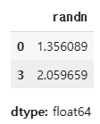
vactor[vactor > vactor.mean()]
vactor[vactor == vactor.max()]
vactor[vactor == vactor.min()]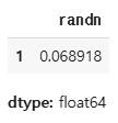
2-2-4. 데이터 수정
vactor[0] = 3.14
vactor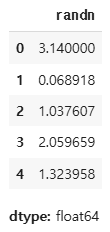
vactor[3:] = np.random.randn(2)
vactor
2-2-5. 데이터 연산
vactor + vactor
vactor - 1.1
vactor * 2
vactor.abs() # 절댓값
2.2.6. 데이터 형 변환
list(vactor)
# [3.14,
#  0.0689180570636732,
#  1.0376065641339183,
#  0.33651530275470876,
#  -0.15040139101998132]

list(vactor.index)
# [0, 1, 2, 3, 4]

list(vactor.items())
# [(0, 3.14),
#  (1, 0.0689180570636732),
#  (2, 1.0376065641339183),
#  (3, 0.33651530275470876),
#  (4, -0.15040139101998132)]
2-3. pd.DataFrame
2-3-1. pd.DataFrame 생성하기
DataFrame은 2차원 구조의 데이터로, 매트릭스 데이터를 말한다.
data = {
    'one': pd.Series([1, 2, 3, 4, 5]),
    'two': pd.Series([10, 20, 30, 40, 50])
}

df = pd.DataFrame(data=data)
df
list(df.index)
# [0, 1, 2, 3, 4]

list(df.columns)
# ['one', 'two']

df.shape
# (5, 2)
2-3-2. 슬라이스 / 인덱스
df['one'][2] # 3
df['two'][2:]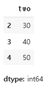
df.iloc[2]
df.iloc[2, 0] # 3
df.iloc[2:4, 1]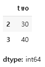
df.loc[2:4, ['two']]

2-3-3. 데이터 수정 및 연산
df['three'] =  df['one'] + df['two']
df['lt_2'] = df['one'] > 2

df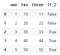
del df['lt_2']
df.pop('three')

df
2-3-4. 데이터 형 변환
df.to_dict()
# {'one': {0: 1, 1: 2, 2: 3, 3: 4, 4: 5},
#  'two': {0: 10, 1: 20, 2: 30, 3: 40, 4: 50}}
df.to_dict('series')
# {'one': 0    1
#  1    2
#  2    3
#  3    4
#  4    5
#  Name: one, dtype: int64,
#  'two': 0    10
#  1    20
#  2    30
#  3    40
#  4    50
#  Name: two, dtype: int64}
df.to_dict('records')
# [{'one': 1, 'two': 10},
#  {'one': 2, 'two': 20},
#  {'one': 3, 'two': 30},
#  {'one': 4, 'two': 40},
#  {'one': 5, 'two': 50}]
df.to_json()
# {"one":{"0":1,"1":2,"2":3,"3":4,"4":5},"two":{"0":10,"1":20,"2":30,"3":40,"4":50}}

df.to_json(orient='records')
# [{"one":1,"two":10},{"one":2,"two":20},{"one":3,"two":30},{"one":4,"two":40},{"one":5,"two":50}]
print(df.to_csv())
# ,one,two
# 0,1,10
# 1,2,20
# 2,3,30
# 3,4,40
# 4,5,50
2-3-5. 통계 데이터
import seaborn as sns

iris = sns.load_dataset("iris")

iris.shape
# (150, 5)

iris.info()
# <class 'pandas.core.frame.DataFrame'>
# RangeIndex: 150 entries, 0 to 149
# Data columns (total 5 columns):
#  #   Column        Non-Null Count  Dtype
# ---  ------        --------------  -----
#  0   sepal_length  150 non-null    float64
#  1   sepal_width   150 non-null    float64
#  2   petal_length  150 non-null    float64
#  3   petal_width   150 non-null    float64
#  4   species       150 non-null    object
# dtypes: float64(4), object(1)
# memory usage: 6.0+ KB
iris.head()
iris.tail()
iris.describe()
iris['species'].describe()
iris[iris['sepal_length'] > 5]
# iris[iris['sepal_length'] > 5] -> 메트릭스(2차원)
# iris[iris['sepal_length'] > 5]['sepal_length'] -> 벡터(1차원)
# iris[iris['sepal_length'] > 5]['sepal_length'].min() -> 스칼라(0차원)
iris[iris['sepal_length'] > 5]['sepal_length'].min()			# 5.1
# iris[iris['sepal_length'] > 5] -> 메트릭스(2차원)
# iris[iris['sepal_length'] > 5].iloc[:,:4] -> 메트릭스(2차원)
# iris[iris['sepal_length'] > 5].iloc[:,:4].median() -> 벡터(1차원)
iris[iris['sepal_length'] > 5].iloc[:,:4].median()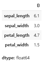
# iris[(iris['sepal_length'] > 5) & (iris['sepal_width'] > 3)].head()
cond1 = iris['sepal_length'] > 5
cond2 = iris['sepal_width'] > 3
cond = cond1 & cond2
iris[cond].shape			# (47, 5)
iris[cond].head()
cond = cond1 | cond2
iris[cond].shape			# (138, 5)
iris[cond].head()
cond3 = iris['species'] == 'setosa'
cond = cond1 & cond2 & cond3
iris[cond.shape]			# (22, 5)
iris[cond].head()
iris[~cond].shape # (128, 5)
iris.select_dtypes(include==np.number).head()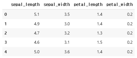
iris.select_dtypes(exclude=np.number).head()
2-4. Pandas 심화
데이터를 분석할 때, 기본적으로 다음과 같은 함수들을 주로 사용하여 데이터를 파악한다.
df.info() 함수를 통해 데이터의 모양(shape), 결측치(null)의 유무, 데이터의 타입, 사용하는 메모리의 양 등을 알 수 있다.
import seaborn as sns

df = sns.load_dataset("titanic")
df.shape						# (891, 15)

df.info()
# <class 'pandas.core.frame.DataFrame'>
# RangeIndex: 891 entries, 0 to 890
# Data columns (total 15 columns):
#  #   Column       Non-Null Count  Dtype
# ---  ------       --------------  -----
#  0   survived     891 non-null    int64
#  1   pclass       891 non-null    int64
#  2   sex          891 non-null    object
#  3   age          714 non-null    float64
#  4   sibsp        891 non-null    int64
#  5   parch        891 non-null    int64
#  6   fare         891 non-null    float64
#  7   embarked     889 non-null    object
#  8   class        891 non-null    category
#  9   who          891 non-null    object
#  10  adult_male   891 non-null    bool
#  11  deck         203 non-null    category
#  12  embark_town  889 non-null    object
#  13  alive        891 non-null    object
#  14  alone        891 non-null    bool
# dtypes: bool(2), category(2), float64(2), int64(4), object(5)
# memory usage: 80.7+ KB

df.head()
df.tail()

df.select_dtypes(include=np.number).describe()		# count, mean, std, min, 25%, 50%, 75%, max
df.select_dtypes(exclude=np.number).describe()		# count, unique, top, freq

df.isnull().sum()
2-4-1. 통계
df_number = df.select_dtypes(include=np.number)
df_number.head()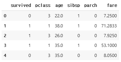
df_number['fare'].mean()		# 32.204207968574636
df_number['fare'].sum()			# 28693.9493
df_number['fare'].median()		# 14.4542
df_number['fare'].max()			# 512.3292
df_number['fare'].min()			# 0.0
df_object = df.select_dtypes(exclude=np.number)
df_object.head()
df_object['sex'].value_counts()
df_object['sex'].unique()		# array(['male', 'female'], dtype=object)
df_object['sex'].nunique()		# 2
2-4-2. map()
map() 함수는 pd.Series()의 데이터를 조작할 때 사용한다.
x = pd.Series({
    'one': 1, 'two': 2, 'three': 3
})
# index: 'one', 'two', 'three' & data: 1, 2, 3

y = pd.Series({
    1: 'a', 2: 'aa', 3: 'aaa'
})
# index: 1, 2, 3 & data: 'a', 'aa', 'aaa'

x.map(y)
"""
gender = {
    'male': 1,
    'female': 2
}
df['gender'] = df['sex'].map(gender)
"""
"""
def gender_map(data):
    if data == 'male':
        return 1
    else:
        return 2

df['gender'] = df['sex'].map(gender_map)
"""
df['gender'] = df['sex'].map(lambda data: 1 if data=='male' else 2)

df[['gender', 'sex']].head()
2-4-3. apply()
apply() 함수는 pd.DataFrame()의 데이터를 조작할 때 사용한다. 이때, axis 변수를 설정해야 한다.
df['new_age'] = df['age'].apply(lambda data: data*10)
df[['new_age', 'age']].head()
df['new_age'] = df.apply(lambda data: data['age'] * 10 if data['sex'] == 'male' else data['age'] * 5, axis=1)
df[['age', 'sex', 'new_age']].head()
# df.select_dtypes(include=np.number).max(axis=0)
"""
def max_value(data):
    return data.max()

df.select_dtypes(include=np.number).apply(max_value, axis=0)
"""
df.select_dtypes(include=np.number).apply(lambda data: data.max(), axis=0)
2-4-4. 집합
df = sns.load_dataset('titanic')
df.shape
# (891, 15)

df.columns
# Index(['survived', 'pclass', 'sex', 'age', 'sibsp', 'parch', 'fare',
#        'embarked', 'class', 'who', 'adult_male', 'deck', 'embark_town',
#        'alive', 'alone'],
#       dtype='object')
df_tmp = df[['survived', 'age', 'fare', 'pclass', 'sex']]
df_tmp.shape			# (891, 4)
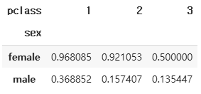
pivot_table() 함수는 데이터 중에서 두 개의 열을 각각 행 index, 열 index로 사용하여 데이터를 조회할 때 사용한다.
파라미터로는 data, values, index, column, aggfunc 등을 갖는다.
- data: pd.DataFrame
- values: 분석하고 싶은 data의 column명
- index: 분석할 때 사용할 기준이 되는 data의 column명
- columns: 분석할 때 사용할 기준이 되는 data의 column명
- aggfunc: 분석할 data의 집계(통계) 함수
pd.pivot_table(
    data=df_tmp,
    values='survived',
    index='sex',
    columns='pclass',
    aggfunc='mean'
)
pd.pivot_table(
    data=df_tmp,
    values='survived',
    index='sex',
    columns='pclass',
    aggfunc=['mean', 'median']
)
'SK네트웍스 Family AI캠프 10기 > Daily 회고' 카테고리의 다른 글
| 17일차. Data Visualization (1) | 2025.02.04 |
|---|---|
| 16일차. Pandas & Data Visualization (0) | 2025.02.03 |
| 13-14일차. 단위 프로젝트(프로그래밍과 데이터 기초) (0) | 2025.01.24 |
| 12일차. Crawling (0) | 2025.01.22 |
| 11일차. Git & Streamlit & Crawling (0) | 2025.01.21 |


