19일 차 회고.
오늘은 배운 것을 다 정리하지 못했다. 토이 프로젝트를 진행하느라 오늘 해야 할 자격증 공부도 다 하지 못해서 주말 동안 블로그를 정리하고 자격증 공부에 조금 더 시간을 써야 할 것 같다.
Numpy 심화부터 수정
1. Machine Learning
1-1. 인공지능(AI; Artificial Intelligence)
인공지능은 인간의 지능으로 할 수 있는 사고, 학습, 자기 개발 등 컴퓨터가 대체할 수 있도록 하는 방법을 연구하는 분야이다.

1-2. 머신러닝(ML; Machine Learning)
머신러닝은 데이터 학습 기반의 인공지능 분야로, 기계가 데이터를 이용해 학습할 수 있도록 하는 알고리즘과 기술을 개발하는 분야이다.
머신러닝 시스템 워크플로우

- 수집
- 머신러닝 학습에 필요한 데이터를 수집하는 단계
- 점검 및 탐색
- 수집된 데이터의 구조, 노이즈 등을 파악하는 단계
- 탐색적 데이터 분석(EDA; Exploratory Data Analysis) 단계
- 전처리 및 정제
- 머신러닝 학습에 알맞게 데이터 정제 및 전처리를 하는 단계
- 모델링 및 훈련
- 적절한 머신러닝 알고리즘을 선택 및 전처리가 완료된 데이터를 이용하여 머신러닝 학습을 진행하는 단계
- 평가
- 테스트 데이터를 통해 모델 학습 평가를 진행하는 단계
- 평가가 좋지 않으면, 다시 머신러닝 학습을 진행한다.
- 배포
- 성공적으로 훈련이 된 것으로 판단될 경우, 완성된 모델을 서비스에 적용하기 위해 운영 및 배포를 진행하는 단계
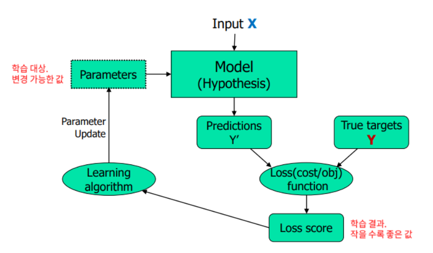
머신러닝 학습 작동 방식
머신러닝은 Loss score를 최소화하는 Parameters를 찾는 과정으로 학습한다.
머신러닝 알고리즘 분류
- 지도학습(Supervised Learning)
- 모델에 주입하는 데이터에 입력값(특성)과 출력값(정답)을 같이 넣어 학습시키는 방식
- 미래 데이터 예측
- 종류
- 분류(classification)
- 회귀(regression)
- 비지도학습(Unsupervised Learning)
- 모델에 입력값(특성)만 넣어 학습시키는 방식
- 데이터의 숨겨진 구조/특징 발견
- 종류
- 클러스터링(clustering)
- 강화학습(Reinforcement Learning)
- 모델에 학습 결과에 따라 보상 또는 벌점을 주어 가장 큰 보상을 받는 방향으로 학습시키는 방식
- 의사결정을 위한 최적의 액션 선택
머신러닝 기본 용어
- Feature
- 독립 변수, 설명 변수
- 학습 데이터의 특성
- Label, Target, Class
- 종속 변수
- 정답 데이터
- Parameter
- 모델이 학습과정에서 업데이트하는 파라미터
- Hyper parameter
- 사용자가 직접 세팅해주는 파라미터
- Loss
- 손실
- 정답값과 예측값의 오차를 표현하는 지표
- Metric
- 평가 지표
- 모델의 성능을 평가할 때, 사용하는 지표
2. scikit-learn
2-1. scikit-learn
Data Cleaning & Feature Engineering
- Data Preprocessing: sklearn.preprocessing
- Feature Selection: sklearn.feature_selection
- Feature Extraction: sklearn.feature_extraction
모델 성능 평가
- 데이터 분리: sklearn.model_selection
- 성능 평가: sklearn.metrics
Supervised Learning
- 앙상블: sklearn.ensemble
- Linear Model: sklearn.linear_molel
- Decision Tree: sklearn.tree
Unsupervised Learning
- Clustering: sklearn.cluster
- Decomposition: sklearn.decomposition
알고리즘 규칙
- 분류 알고리즘: __Classifier
- ex. DecisionTreeClassifier
- 회귀 알고리즘: __Regressor
- ex. DecisionTreeRegressor
2-2. 머신러닝 워크플로우
Global Variables
import easydict
args = easydict.EasyDict()		# args -> 사용할 변수 저장

args.SEED = 10				# seed: random 값 지정
args.target_col = 'target'
Load Dataset
from sklearn.datasets import load_breast_cancer

breast_cancer = load_breast.cancer()
학습용/검증용 데이터 분리
import numpy as np
import pandas as pd

from sklearn.model_selection import train_test_split
df_cancer = pd.DataFrame(breast_cancer.data, columns=breast_cancer, feature_names)

df_cancer[args.target_col] = breast_cancer[args.target_col]

train, test = train_test_split(df_cancer, random_state=args.SEED)

train.shape, test.shape				# ((426, 31), (143, 31))
데이터 점검 및 탐색
train.head()
train.tail()

train.info()

train.describe()
전처리 및 정제
x_train, x_test = train.drop(args.target_col, axis=1), test.drop(args.target_col, axis=1)
y_train, y_test = train[args.target_col], test[args.target_col]

x_train.shape, y_train.shape			# ((426, 30), (426,))

x_test.shape, y_test.shape			# ((143, 30), (143,))
from sklearn.preprocessing import StandardScaler

scaler = StandardScaler()

train_scaled = scaler.fit_transform(x_train)
test_scaled = scaler.transform(x_test)
모델링 및 훈련
from sklearn.linear_model import LogisticRegression

lr_clf = LogisticRegression()

lr_clf.fit(x_train, y_train)
평가
from sklearn.metrics import accuracy_score

pred = lr_clf.predict(x_test)

accuracy_score(y_test, pred)			# 0.9230769230769231
3. Numpy
3-1. 선형대수학
scaler
scaler는 0차원 물리량이다.
vector
vector는 1차원 물리량으로, scaler의 집합이다.
matrix
matrix는 2차원 물리량으로, vector의 집합이다.
- diagonal matrix
- 주대각선 성분이 아닌 모든 성분이 0인 square matrix
- square matrix
- n개의 행과 n개의 열을 가지는 정사각형 matrix
- identity matrix
- diagonal matrix이면서 주대각선 성분이 모두 1인 square matrix
- zero matrix
- transpose matrix
- symmetric matrix
- square matrix이면서 자신의 transpose matrix와 똑같은 matrix
- orthogonal matrix
- 어떤 matrix의 행 벡터와 열 벡터가 유클리드 공간의 정규 직교를 이루는 matrix
직교(orthogonal)
두 벡터가 서로 직교한다는 것은 두 벡터가 이루는 각이 90도인 경우를 말한다.
선형 독립(linearly independence)
두 벡터가 선형 독립이라는 것은 두 벡터가 일직선 상에 놓이지 않고 서로 독립적인 방향을 가지고 있다는 것을 말한다.
선형 종속(linearly dependence)
두 벡터가 선형 종속이라는 것은 두 벡터가 일직선 상에 놓여있다는 것을 말한다.
Vector 연산
- Norm
- 벡터의 크기
- L1(Manhatten) Norm
- 두 개의 벡터를 빼고, 절댓값을 취한 뒤, 합한 것
- L2(Euclidean) Norm
- 두 개의 벡터의 각 원소를 빼고, 제곱을 하고, 합치고 루트를 씌운 것
- 내적
- 벡터의 내적은 항상 scaler이다.
- 벡터 간의 유사도(상관계수) 크기로 해석할 수 있다.
Matrix 연산
- 행렬의 덧셈과 뺄셈

- 행렬의 스칼라 곱

- 행렬의 곱

- 선형변환(Linear Transformation)

3-2. Numpy
Numpy는 C언어로 구현된 Python 라이브러리로, 벡터 및 행렬 연산에 주로 사용된다.
numpy.ndarray
- ndarray.ndim
- array의 차원
- ndarray.shape
- array의 크기를 나타내는 정수 튜플
- ndarray.size
- array의 요소 총 개수
- ndarray.dtype
- array의 요소의 데이터 타입
vector, matrix
import numpy as np

lst = [1, 2, 3, 4, 5]
vector = np.array(lst)

lst = [
    [1, 2, 3],
    [4, 5, 6]
]
matrix = np.array(lst)
3-3. Numpy 기초
import numpy as np
배열 생성
lst = [
    [1, 2, 3],
    [4, 5, 6]
arr = np.array(lst)

arr.ndim				# 2
arr.shape				# (2, 3)
arr.size				# 6
특수 배열 생성
np.arange(10)
# array([0, 1, 2, 3, 4, 5, 6, 7, 8, 9])

np.arange(5, 10)
# array([5, 6, 7, 8, 9])

rg = np.random.default_rng(1)
np.floor(10 * rg.random((2, 2)))
# array([[5., 9.],
#        [1., 0.]])

np.zeros((5, 3))
# array([[0., 0., 0.],
#        [0., 0., 0.],
#        [0., 0., 0.],
#        [0., 0., 0.],
#        [0., 0., 0.]])

np.ones((2, 3))
# array([[1., 1., 1.],
#        [1., 1., 1.]])

np.full((2, 3), 5)
# array([[5, 5, 5],
#        [5, 5, 5]])

np.eye(2)
# array([[1., 0.],
#        [0., 1.]])
배열 결합
arr1 = np.array([[1, 1],
               [2, 2]])
arr2 = np.array([[3, 3],
               [4, 4]])

arrv = np.vstack((arr1, arr2))
arrv.shape				# (4, 2)
arrv
# array([[1, 1],
#        [2, 2],
#        [3, 3],
#        [4, 4]])

arrh = np.hstack((arr1, arr2)
arrh.shape				# (2, 4)
arrh
# array([[1, 1, 3, 3],
#        [2, 2, 4, 4]])
배열의 차원 변환
arr = np.arange(6)
arr.base
arr.shape				# (6,)
arr
# array([0, 1, 2, 3, 4, 5])

# arr[:, np.newaxis].shape		# (6, 1)
arr1 = np.expand_dims(arr, axis=1)
arr1.shape				# (6, 1)
arr1
# array([[ 0],
#        [ 1],
#        [ 2],
#        [ 3],
#        [ 4],
#        [ 5]])

arr2 = np.expand_dims(arr, axis=0)
arr2.shape				# (1, 6)
arr2
# array([[ 0,  1,  2,  3,  4, 5]])
arr
# array([0, 1, 2, 3, 4, 5])

arr.resize((3, 2))
arr
# array([[0, 1],
#        [2, 3],
#        [4, 5]])

arr.ravel()
# array([0, 1, 2, 3, 4, 5])

arr.T
# array([[0, 2, 4],
#        [1, 3, 5]])

arr.reshape(2, -1)
# array([[0, 1, 2],
#        [3, 4, 5]])

arr = arr.reshape(2, 3)
arr
# array([[0, 1, 2],
#        [3, 4, 5]])

arr.base
# array([[0, 1],
#        [2, 3],
#        [4, 5]])

arr.view()
# array([[0, 1, 2],
#        [3, 4, 5]])

arr
# array([[0, 1, 2],
#        [3, 4, 5]])

arr.shape				# (2, 3)
데이터 타입
arr = np.arange(6)
type(arr)
# numpy.ndarray

arr
# array([0, 1, 2, 3, 4, 5])

arr.dtype
# dtype('int64')

arr = arr.astype(np.float32)			# 데이터 타입 변환
arr.dtype
# dtype('float32')

arr
# arr([0., 1., 2., 3., 4., 5.])			# 데이터 타입 변환

arr = np.int8(arr)
arr.dtype
# dtype('int8')
np.iinfo(np.uint8)
# iinfo(min=0, max=255, dtype=uint8)

np.iinfo(np.int32)
# iinfo(min=-2147483648, max=2147483647, dtype=int32)

np.iinfo(np.int64)
# iinfo(min=-9223372036854775808, max=9223372036854775807, dtype=int64)
슬라이싱 / 인덱싱
arr = np.array([1, 2, 3])
arr
# array([1, 2, 3])

arr[1], arr[-1]				# (2, 3)
arr[0:2]				# array([1, 2])
arr[::-1]				# array[::-1]
lst = [
    [1, 2, 3],
    [4, 5, 6],
    [7, 8, 9]
]
arr = np.array(lst)
arr.shape				# (3, 3)
arr
# array([[1, 2, 3],
#        [4, 5, 6],
#        [7, 8, 9]])

arr[0, :]				# array([1, 2, 3])
arr[:, 0]				# array([1, 4, 7])

arr[:, ::-1]
# array([[3, 2, 1],
#        [6, 5, 4],
#        [9, 8, 7]])

arr[0, :] = [11, 12, 13]
arr
# array([[11, 12, 13],
#        [ 4,  5,  6],
#        [ 7,  8,  9]])
배열 조건 연산
arr = np.array([[1, 2, 3], [4, 5, 6], [7, 8, 9]])
arr
# array([[1, 2, 3],
#        [4, 5, 6],
#        [7, 8, 9]])

arr < 5
# array([[ True,  True,  True],
#        [ True, False, False],
#        [False, False, False]])

arr[arr < 5]				# array([1, 2, 3, 4])

cond = (arr >= 5)
arr[cond]				# array([5, 6, 7, 8, 9])
arr
# array([[1, 2, 3],
#        [4, 5, 6],
#        [7, 8, 9]])

np.any(arr > 8)				# True

np.all(arr >= 1)			# True

np.where(arr > 5, 1, 0)
# array([[0, 0, 0],
#        [0, 0, 1],
#        [1, 1, 1]])

np.clip(arr, 3, 6)
# array([[3, 3, 3],
#        [4, 5, 6],
#        [6, 6, 6]])
arr = np.array([np.inf, np.nan, 3, 4, 5, np.nan, 6, 7])
arr
# array([inf, nan, 3., 4., 5., nan, 6., 7.])

is_inf = np.isinf(arr)
is_inf
# array([ True, False, False, False, False, False, False, False])

is_nan = np.isnan(arr)
np.any(is_nan), np.all(is_nan)			# (True, False)

np.isfinite(arr)
# array([False, False,  True,  True,  True, False,  True,  True])

arr[np.isfinite(arr) == False] = 0
arr
# array([0., 0., 3., 4., 5., 0., 6., 7.])
마스킹
lst = [
    [1, 2, 3],
    [4, 5, 6],
    [7, 8, 9]
]
arr = np.array(lst)
arr.shape(3, 3)
arr
# array([[1, 2, 3],
#        [4, 5, 6],
#        [7, 8, 9]])

mask = [True, False, True]
arr[:, mask]
# array([[1, 3],
#        [4, 6],
#        [7, 9]])

mask = arr > 5
arr[mask]
# array([6, 7, 8, 9])
Broadcasting
arr1 = np.array([1.0, 2.0, 3.0])
arr2 = np.array([2.0, 2.0, 2.0])
arr1 * arr2				# array([2., 4., 6.])

arr1 * 2				# array([2., 4., 6.])
arr1 = np.array([
          [ 0.0,  0.0,  0.0],
          [10.0, 10.0, 10.0],
          [20.0, 20.0, 20.0],
          [30.0, 30.0, 30.0]
        ])
arr2 = np.array([1.0, 2.0, 3.0])
arr1 + arr2
# array([[ 1.,  2.,  3.],
#        [11., 12., 13.],
#        [21., 22., 23.],
#        [31., 32., 33.]])
arr1 = np.array([0.0, 10.0, 20.0, 30.0])
arr2 = np.array([1.0, 2.0, 3.0])
arr1[:, np.newaxis] + arr2
# array([[ 1.,  2.,  3.],
#        [11., 12., 13.],
#        [21., 22., 23.],
#        [31., 32., 33.]])
3-4. Numpy 심화
Broadcasting
Norm
덧셈과 뺄셈
내적
- 1차원 배열 내적
x = np.array([1, 2, 3])
y = np.array([4, 5, 6])

x @ y				# 32
np.dot(x, y)			# 32
x.dot(y.T)			# 32
y.dot(x.T) # 32- 2차원 배열 내적
x = np.array([[1], [2], [3]])
y = np.array([[4], [5], [6]])

x.T				# array([[1, 2, 3]])

x.T @ y				# array([[32]])
np.dot(x.T, y)			# array([[32]])

y.T				# array([[4, 5, 6]])

x @ y.T
# array([[ 4,  5,  6],
#        [ 8, 10, 12],
#        [12, 15, 18]])
np.dot(x, y.T)
# array([[ 4,  5,  6],
#        [ 8, 10, 12],
#        [12, 15, 18]])
역행렬
from numpy.linalg import inv

x = np.array([[1, 2, 3], [1, 0, 0], [0, 0, 1]])
x.shape				# (3, 3)

y = inv(x)
y
# array([[ 0. ,  1. ,  0. ],
#        [ 0.5, -0.5, -1.5],
#        [ 0. ,  0. ,  1. ]])

x.dot(y)
# array([[1., 0., 0.],
#        [0., 1., 0.],
#        [0., 0., 1.]])
난수
import matplotlib.pyplot as plt

plt.style.use('default')
plt.rcParams['figure.figsize'] = (6, 3)
plt.rcParams['font.size'] = 12
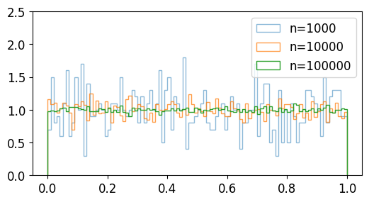
- rand
np.random.seed(0)

# 난수 1000개 생성
a = np.random.rand(1000)
# 난수 10000개 생성
b = np.random.rand(10000)
# 난수 100000개 생성
c = np.random.rand(100000)

plt.hist(a, bins=100, density=True, alpha=0.5, histtype='step', label='n=1000')
plt.hist(b, bins=100, density=True, alpha=0.75, histtype='step', label='n=10000')
plt.hist(c, bins=100, density=True, alpha=1.0, histtype='step', label='n=100000')

plt.ylim(0, 2.5)
plt.legend()
plt.show()
- randint
np.random.seed(0)

# a는 (0, 10) 범위의 임의의 정수 1000개
a = np.random.randint(0, 10, 1000)
# b는 (10, 20) 범위의 임의의 정수 1000개
b = np.random.randint(10, 20, 1000)
# c는 (0, 20) 범위의 임의의 정수 1000개
c = np.random.randint(0, 20, 1000)

plt.hist(a, bins=100, density=False, alpha=0.5, histtype='step', label='0<=randint<10')
plt.hist(b, bins=100, density=False, alpha=0.75, histtype='step', label='10<=randint<20')
plt.hist(c, bins=100, density=False, alpha=1.0, histtype='step', label='0<=randint<20')

plt.ylim(0, 150)
plt.legend()
plt.show()

- randn
np.random.seed(0)

# a는 평균과 표준편차가 각각 0,1인 정규분포의 난수 100000개
a = np.random.randn(100000)
# b는 평균과 표준편차가 각각 -1,2인 정규분포의 난수 100000개
b = 2 * np.random.randn(100000) - 1
# c는 평균과 표준편차가 각각 2,4인 정규분포의 난수 100000개
c = 4 * np.random.randn(100000) + 2

plt.hist(a, bins=100, density=True, alpha=0.5, histtype='step', label='(mean, stddev)=(0, 1)')
plt.hist(b, bins=100, density=True, alpha=0.75, histtype='step', label='(mean, stddev)=(-1, 2)')
plt.hist(c, bins=100, density=True, alpha=1.0, histtype='step', label='(mean, stddev)=(2, 4)')

plt.xlim(-15, 25)
plt.legend()
plt.show()

- standard_normal
np.random.seed(0)

# 표준정규분포를 갖는 난수 1000개
a = np.random.standard_normal(1000)
# 표준정규분포를 갖는 난수 10000개
b = np.random.standard_normal(10000)
# 표준정규분포를 갖는 난수 100000개
c = np.random.standard_normal(100000)

plt.hist(a, bins=100, density=True, alpha=0.5, histtype='step', label='n=1000')
plt.hist(b, bins=100, density=True, alpha=0.75, histtype='step', label='n=10000')
plt.hist(c, bins=100, density=True, alpha=1.0, histtype='step', label='n=100000')

plt.legend()
plt.show()

- normal
np.random.seed(0)

# 평균 0, 표준편차 1인 정규분포를 갖는 난수 500개
a = np.random.normal(0, 1, 500)
# 평균 1.5, 표준편차 1.5인 정규분포를 갖는 난수 5000개
b = np.random.normal(1.5, 1.5, 5000)
# 평균 3.0, 표준편차 2.0인 정규분포를 갖는 난수 50000개
c = np.random.normal(3.0, 2.0, 50000)

plt.hist(a, bins=100, density=True, alpha=0.75, histtype='step', label=r'N(0, $1^2$)')
plt.hist(b, bins=100, density=True, alpha=0.75, histtype='step', label=r'N(1.5, $1.5^2$)')
plt.hist(c, bins=100, density=True, alpha=0.75, histtype='step', label=r'N(3.0, $2.0^2$)')

plt.legend()
plt.show()

- random_sample
np.random.seed(0)

a = np.random.random_sample(100000)
b = 1.5 * np.random.random_sample(100000) - 0.75
c = 2 * np.random.random_sample(100000) - 1

plt.hist(a, bins=100, density=True, alpha=0.75, histtype='step', label='[0, 1)')
plt.hist(b, bins=100, density=True, alpha=0.75, histtype='step', label='[-0.75, 0.75)')
plt.hist(c, bins=100, density=True, alpha=0.75, histtype='step', label='[-1, 1)')

plt.ylim(0.0, 1.2)
plt.legend()
plt.show()

- choice
np.random.seed(0)

# np.arange(10)에서 1000개 생성
a = np.random.choice(10, 1000)
# [0, 1, 2, 4, 8]에서 1000개 생성
b = np.random.choice([0, 1, 2, 4, 8], 1000)

plt.hist(a, bins=100, density=False, alpha=0.75, histtype='step', label='Sample np.arange(10)')
plt.hist(b, bins=100, density=False, alpha=0.75, histtype='step', label='Sample [0, 1, 2, 4, 8]')

plt.ylim(0, 300)
plt.legend()
plt.show()

상수
- inf
- (양의) 무한대 부동소수점 표현
np.int # inf- nan
- Not a Number
np.nan # nan- newaxis
- 차원 추가
4. Feature Extraction
4-1. 라이브러리 로드
# 구글 드라이브 연결
from google.colab import drive

drive.mount('/content/data')
데이터 분석용 라이브러리
import pandas as pd
import numpy as np

import logging
logging.getLogger('matplotlib.font_manager').setLevel(logging.ERROR)
데이터 시각화용 라이브러리
import matplotlib.pyplot as plt
import matplotlib as mpl
import seaborn as sns

# 브라우저에서 바로 그리기
%matplotlib inline

# 그래프에 retina display 적용
%config InlineBackend.figure_format = 'retina'

# 유니코드에서 음수 부호 설정
mpl.rc('axes', unicode_minus=False)
4-2. 데이터 로드
'SK네트웍스 Family AI캠프 10기 > Daily 회고' 카테고리의 다른 글
| 21일차. Supervised Learning - Regression & Classification (0) | 2025.02.10 |
|---|---|
| 20일차. Feature Extraction & Data Encoding (0) | 2025.02.07 |
| 18일차. Data Visualization(Seaborn) & Data Cleaning (0) | 2025.02.05 |
| 17일차. Data Visualization (1) | 2025.02.04 |
| 16일차. Pandas & Data Visualization (0) | 2025.02.03 |


