더보기
22일 차 회고.
어제부터 토이 프로젝트에 대해서 계속 생각을 했는데 빠지는 것이 좋을 것 같다는 결론을 내리게 되었다. 팀원분들 모두 좋으셨지만 이대로는 배우는 것도 개발하는 것도 이도저도 아니게 될 것 같아서 이번 1차 애자일까지만 참여하기로 했다. 수업도 따라가기 힘들어지고 자격증 준비와 코딩테스트 공부도 해야 하기 때문에 이게 제일 좋은 선택인 것 같다.
1. Supervised Learning - Classification
1-1. Multiclass Classification
가능도(Likehood)

- 확률(Probability)
- 확률 분포가 고정된 상태에서, 관측되는 사건이 변화되는 경우
- 가능도(Likelihood)
- 관측되는 사건이 고정된 상태에서, 확률 분포가 변화되는 경우
최대가능도 추정량(MLE; Maximum Likelihood Estimator)
- 최대가능도 추정은 주어진 관측값에 대한 총 가능도를 최대로 하는 확률분포를 찾는 것을 말한다.
Binary Classification - Sigmoid
import numpy as np
import matplotlib.pyplot as plt

def sigmoid(x):
    return 1 / (1 + np.exp(-x))

x = np.arange(-5.0, 5.0, 0.1)
y = sigmoid(x)
plt.plot(x, y)
plt.ylim(-0.1, 1.1)
plt.show()
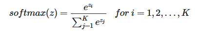
Multiclass Classification - SoftMax
import numpy as np
import matplotlib.pyplot as plt

def softmax(x):
    e_x = np.exp(x - np.max(x))
    return e_x / e_x.sum()

x = np.array([1.0, 1.0, 2.0])
y = softmax(x)

ratio = y
labels = y

plt.pie(ratio.labels=labels, startangle=90)
plt.show()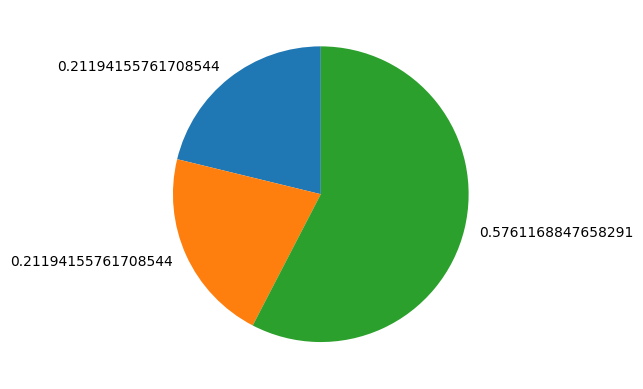
코드 구현
- Load Data
from sklearn.datasets import load_digits
from sklearn.model_selection import train_test_split

digits = load_digits()

# features: target을 예측하기 위해 필요한 데이터
data = digits.data
# target: 예측할 데이터
target = digits.target

SEED = 42
# 모델 학습의 평가를 위한 테스트 데이터 분리
x_train, x_valid, y_train, y_valid = train_test_split(data, target, random_state=SEED)
import matplotlib as mpl
import matplotlib.pyplot as plt
digit_img = x_valid[0].reshape(8, 8)
plt.imshow(digit_img, cmap="gray")
plt.axis("off")
plt.show()
- Modeling
from sklearn.tree import DecisionTreeClassifier

# 모델 정의: max_depth -> 하이퍼 파라미터
tree = DecisionTreeClassifier(max_depth = 5 , random_state=SEED)
# 모델 학습: feature(x_train) & target(y_train) -> Supervised Learning
tree.fit(x_train,y_train)
# 모델 예측: predict() -> int / predict_proba() -> probability
pred = tree.predict(x_valid)- 결과
from sklearn.metrics import classification_report

print(classification_report(y_valid, pred))

#               precision    recall  f1-score   support
#
#            0       1.00      0.91      0.95        43
#            1       0.32      0.32      0.32        37
#            2       0.56      0.66      0.60        38
#            3       0.87      0.85      0.86        46
#            4       0.80      0.78      0.79        55
#            5       0.73      0.19      0.30        59
#            6       0.95      0.89      0.92        45
#            7       0.90      0.68      0.78        41
#            8       0.37      0.61      0.46        38
#            9       0.52      0.85      0.65        48
#
#     accuracy                           0.67       450
#    macro avg       0.70      0.67      0.66       450
# weighted avg       0.71      0.67      0.66       450
from sklearn.metrics import confusion_matrix
import seaborn as sns
norm_conf_mx = confusion_matrix(y_valid, pred, normalize="true")
plt.figure(figsize=(7,5))
sns.heatmap(norm_conf_mx, annot=True, cmap="coolwarm", linewidth=0.5)
plt.xlabel('Predicted')
plt.ylabel('Actual')
plt.show()
- 평가
from sklearn.metrics import f1_score

# micro: 전체 클래스에 대하여 TP/FP/FN을 구한 뒤에 F1-Score 계산
f1_score(y_valid, pred, average="micro")
# 0.6688888888888889

# macro: 각 클래스에 대하여 F1-Score을 계산한 뒤에 산술 평균 계산
f1_score(y_valid, pred, average="macro")
# 0.6620047429878985

# weighted: 각 클래스에 대하여 F1-Score을 계산한 뒤에 각 클래스가 차지하는 비율에 따라 가중 평균 계산
f1_score(y_valid, pred, average="weighted")
# 0.6616398619763888- softmax
x = tree.predict_proba(x_valid)[0]

y = softmax(x)

ratio = y
labels = [0,1,2,3,4,5,6,7,8,9]

plt.pie(ratio, labels=labels, shadow=True, startangle=90)
plt.show()
2. Supervised Learning - Ensemble
1-1. 필수 라이브러리 임포트
!pip install --upgrade joblib==1.1.0
!pip install --upgrade scikit-learn==1.1.3
!pip install mglearn

import logging

logging.getLogger('matplotlib.font_manager').setLevel(logging.ERROR)

import mglearn

from sklearn.model_selection import train_test_split

import pandas as pd
import numpy as np

import matplotlib.pyplot as plt
import matplotlib as mpl
import seaborn as sns

%matplotlib inline
1-2. 앙상블(Ensemble)
앙상블은 여러 머신러닝 모델을 연결하여 더 강력한 모델을 만드는 기법이다.
Bagging
- Bagging
- 데이터로부터 복원추출을 통해 n개의 bootstrap sample 생성
- 해당 sample에 대해 모델(Decision Tree) 학습
- 앞의 과정을 반복한 후, 최종 Bagging 모델 정의
- Random Forest
- 랜덤하게 일부 sample과 feature를 뽑아 여러 개의 tree를 만들어 ensemble하는 모델
- Decision Tree는 overfitting될 확률이 높기 때문에, Random Forest를 통해 이를 회피한다.
from sklearn.ensemble import RandomForestClassifier
from sklearn.datasets import make_moons

X, y = make_moons(n_samples=100, noise=0.25, random_state=3)

X_tr, X_te, y_tr, y_te = train_test_split(X, y, stratify=y, random_state=42)

# n_estimators: Decision Tree 모델 개수
forest = RandomForestClassifier(n_estimators=5, random_state=2).fit(X_tr, y_tr)

fig, axes = plt.subplots(2, 3, figsize=(20,10))

for i, (ax, tree) in enumerate(zip(axes.ravel(), forest.estimators_)):
  ax.set_title(f"tree {i}")
  mglearn.plots.plot_tree_partition(X, y, tree, ax=ax)

mglearn.plots.plot_2d_separator(forest, X, fill=True, ax=axes[-1,-1], alpha=0.4)
axes[-1,-1].set_title("forest")
mglearn.discrete_scatter(X[:, 0], X[:, 1], y)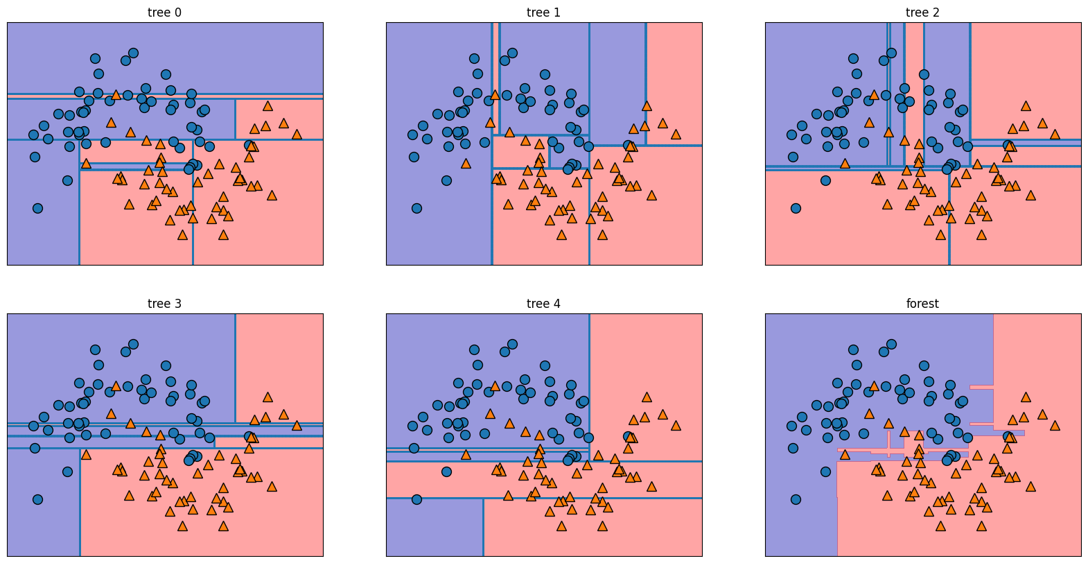
from sklearn.datasets import load_breast_cancer

cancer = load_breast_cancer()
X_tr, X_te, y_tr, y_te = train_test_split(cancer.data, cancer.target, stratify=cancer.target, random_state=42)

forest = RandomForestClassifier(n_estimators=100, random_state=0).fit(X_tr, y_tr)
print(f'훈련용 평가지표: {forest.score(X_tr, y_tr)} / 테스트용 평가지표: {forest.score(X_te, y_te)}')
# 훈련용 평가지표: 1.0 / 테스트용 평가지표: 0.958041958041958

hp = {
    "random_state" : 0,
    "max_features" : "sqrt",
    "n_estimators" : 100,
    "max_depth" : 10,
    "min_samples_split" : 10,
    "min_samples_leaf" : 3,
}
forest = RandomForestClassifier(**hp).fit(X_tr, y_tr)
print(f'훈련용 평가지표: {forest.score(X_tr, y_tr)} / 테스트용 평가지표: {forest.score(X_te, y_te)}')
# 훈련용 평가지표: 0.9882629107981221 / 테스트용 평가지표: 0.958041958041958
Boosting
- Boosting
- weak learner를 생성한 후, error 계산
- error에 기여한 sample마다 다른 가중치를 주고 해당 error를 감소시키는 새로운 모델 학습
- 앞의 과정을 반복한 후, 최종 Boosting 모델 정의
- Gradient Boost
- max_depth를 1 ~ 5 이하로 설정하여 약한 트리들을 만들어 학습하는 알고리즘
from sklearn.ensemble import GradientBoostingRegressor, GradientBoostingClassifier
from sklearn.datasets import load_breast_cancer

cancer = load_breast_cancer()
X_tr, X_te, y_tr, y_te = train_test_split(cancer.data, cancer.target, stratify=cancer.target, random_state=42)

gradient = GradientBoostingClassifier(random_state=0).fit(X_tr, y_tr)
print(f'훈련용 평가지표: {gradient.score(X_tr, y_tr)} / 테스트용 평가지표: {gradient.score(X_te, y_te)}')
# 훈련용 평가지표: 1.0 / 테스트용 평가지표: 0.958041958041958

hp = {
    "random_state" : 0,
    "max_depth" : 1,
    "n_estimators" : 100
}
gradient = GradientBoostingClassifier(**hp).fit(X_tr, y_tr)
print(f'훈련용 평가지표: {gradient.score(X_tr, y_tr)} / 테스트용 평가지표: {gradient.score(X_te, y_te)}')
# 훈련용 평가지표: 0.9882629107981221 / 테스트용 평가지표: 0.958041958041958

hp = {
    "random_state" : 0,
    "max_depth" : 1,
    "n_estimators" : 100,
    "learning_rate" : 0.2,			# 보정 강도
}
gradient = GradientBoostingClassifier(**hp).fit(X_tr, y_tr)
print(f'훈련용 평가지표: {gradient.score(X_tr, y_tr)} / 테스트용 평가지표: {gradient.score(X_te, y_te)}')
# 훈련용 평가지표: 0.9953051643192489 / 테스트용 평가지표: 0.965034965034965- XGBoost
- Gradient Boost를 병렬 학습이 지원되도록 구현한 라이브러리
from xgboost import XGBClassifier, plot_importance

hp = {
    "random_state" : 42
}

xgb = XGBClassifier(**hp).fit(X_tr, y_tr)
print(f'훈련용 평가지표: {xgb.score(X_tr, y_tr)} / 테스트용 평가지표: {xgb.score(X_te, y_te)}')
# 훈련용 평가지표: 1.0 / 테스트용 평가지표: 0.965034965034965

# overfitting 방지
# - learning_rate 낮추기 & n_estimators 높이기
# - max_depth: 낮추기
# - min_child_weight 높이기
# - gamma 높이기
hp = {
    "random_state" : 42,
    "max_depth" : 2,
    "n_estimators" : 200,
    "learning_rate": 0.01,
    "min_child_weight": 2,
    "gamma": 1
}
xgb = XGBClassifier(**hp).fit(X_tr, y_tr)
print(f'훈련용 평가지표: {xgb.score(X_tr, y_tr)} / 테스트용 평가지표: {xgb.score(X_te, y_te)}')
# 훈련용 평가지표: 0.9812206572769953 / 테스트용 평가지표: 0.951048951048951
import matplotlib.pyplot as plt
plot_importance(xgb)
plt.show()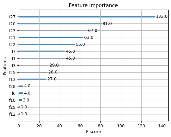
- Light GBM
- 리프 기준 분할 방식을 사용한다.
- 트리의 균형을 맞추지 않고 최대 손실 값을 갖는 리프 노드를 지속적으로 분할하면서 깊고 비대칭적인 트리를 생성한다.
- XGBoost에 비해 빠르며, 예측 오류 손실을 최소화할 수 있다.
from lightgbm import LGBMClassifier, plot_importance

hp = {
    "random_state" : 42
}
lgb = LGBMClassifier(**hp).fit(X_tr, y_tr)
print(f'훈련용 평가지표: {lgb.score(X_tr, y_tr)} / 테스트용 평가지표: {lgb.score(X_te, y_te)}')
# 훈련용 평가지표: 1.0 / 테스트용 평가지표: 0.965034965034965

hp = {
    "random_state" : 42,
    "max_depth" : 2,
    "n_estimators" : 100,
    "learning_rate": 0.01,
}
lgb = LGBMClassifier(**hp).fit(X_tr, y_tr)
print(f'훈련용 평가지표: {lgb.score(X_tr, y_tr)} / 테스트용 평가지표: {lgb.score(X_te, y_te)}')
# 훈련용 평가지표: 0.971830985915493 / 테스트용 평가지표: 0.951048951048951
plot_importance(lgb)
plt.show()
- Catboost
- 범주형 feature가 많을 경우 사용한다.
!pip install catboost

from catboost import CatBoostClassifier

hp = {
    "random_state" : 42,
    "verbose" : 0 # 부스팅 단계 출력 비활성화
}
cat = CatBoostClassifier(**hp).fit(X_tr, y_tr)
print(f'훈련용 평가지표: {cat.score(X_tr, y_tr)} / 테스트용 평가지표: {cat.score(X_te, y_te)}')
# 훈련용 평가지표: 1.0 / 테스트용 평가지표: 0.965034965034965

hp = {
    "random_state" : 42,
    "max_depth" : 2,
    "n_estimators" : 100, # 수행할 부스팅 단계 수
    "verbose" : 0 # 부스팅 단계 출력 비활성화
}
cat = CatBoostClassifier(**hp).fit(X_tr, y_tr)
print(f'훈련용 평가지표: {cat.score(X_tr, y_tr)} / 테스트용 평가지표: {cat.score(X_te, y_te)}')
# 훈련용 평가지표: 0.9882629107981221 / 테스트용 평가지표: 0.965034965034965
feature_importance = cat.feature_importances_
sorted_idx = np.argsort(feature_importance)
fig = plt.figure(figsize=(12, 6))
plt.barh(range(len(sorted_idx)), feature_importance[sorted_idx], align='center')
plt.yticks(range(len(sorted_idx)), np.array(range(len(X_tr)))[sorted_idx])
plt.title('Feature Importance')
Voting
다른 종류의 모델들의 예측값을 합쳐 최종 결과를 도출해 내는 모델
- Hard Voting
- 모델들의 예측 결괏값을 다수결을 통해 최종 class 결정
- Soft Voting
- 모델들의 예측 결괏값의 평균으로 최종 class 결정
from sklearn.ensemble import VotingClassifier
from sklearn.neural_network import MLPClassifier
from sklearn.linear_model import LogisticRegression
from sklearn.ensemble import RandomForestClassifier

SEED = 42
estimators = [
    ( "mlp" , MLPClassifier(max_iter=1000,random_state=SEED) ),
    ( "lr" , LogisticRegression(random_state=SEED) ),
    ( "rf" , RandomForestClassifier(random_state=SEED) )
]

hp = {
    "estimators" : estimators,
    "voting" : "hard"
}
vot = VotingClassifier(**hp).fit(X_tr, y_tr)
print(f'훈련용 평가지표: {vot.score(X_tr, y_tr)} / 테스트용 평가지표: {vot.score(X_te, y_te)}')
# 훈련용 평가지표: 0.9647887323943662 / 테스트용 평가지표: 0.9370629370629371

hp = {
    "estimators" : estimators,
    "voting" : "soft"
}
vot = VotingClassifier(**hp).fit(X_tr, y_tr)
print(f'훈련용 평가지표: {vot.score(X_tr, y_tr)} / 테스트용 평가지표: {vot.score(X_te, y_te)}')
# 훈련용 평가지표: 0.9694835680751174 / 테스트용 평가지표: 0.9440559440559441
Stacking
개별적인 모델들이 학습하여 예측한 데이터를 기반으로 메타 모델을 만들어 예측하는 모델
- training dataset을 이용하여 sub model 예측 결과를 생성한다.
- 앞의 output 결과를 이용하여 training data로 사용하여 meta learner 모델을 생성한다.
from sklearn.ensemble import StackingClassifier
from sklearn.neural_network import MLPClassifier
from sklearn.linear_model import LogisticRegression
from sklearn.ensemble import RandomForestClassifier

SEED = 42
estimators = [
    ( "mlp" , MLPClassifier(max_iter=1000,random_state=SEED) ),
    ( "lr" , LogisticRegression(random_state=SEED) ),
    ( "rf" , RandomForestClassifier(random_state=SEED) )
]

hp = {
    "estimators" : estimators,
    "final_estimator" : LogisticRegression(random_state=SEED)
}

stack = StackingClassifier(**hp,n_jobs=-1).fit(X_tr, y_tr)	# n_jobs: -1(현재 사용 가능한 코어) 권장
print(f'훈련용 평가지표: {stack.score(X_tr, y_tr)} / 테스트용 평가지표: {stack.score(X_te, y_te)}')
# 훈련용 평가지표: 0.9835680751173709 / 테스트용 평가지표: 0.965034965034965
3. Hyper Parameter Optimization
3-1. Parameter
Model Parameters
- 모델 학습을 통해서 최종적으로 찾게 되는 파라미터
- 모델이 학습을 하며 파라미터 값을 변경한다.
Hyper Parameters
- 모델 학습을 효율적으로 할 수 있게 사전에 정의하는 파라미터
- 최적의 학습 모델을 구현하기 위해 사용자가 지정할 수 있다.
3-2. HPO 탐색 방법
Import Library
import numpy as np
import pandas as pd

from sklearn.metrics import classification_report,confusion_matrix
from sklearn.metrics import roc_auc_score

%matplotlib inline

import warnings				# `do not disturbe` mode
warnings.filterwarnings('ignore')
Load Data
import seaborn as sns

df = sns.load_dataset('titanic')
cols = ["age","sibsp","parch","fare"]
features = df[cols]
target = df["survived"]
Data Encoding
from sklearn.preprocessing import OneHotEncoder

cols = ["pclass","sex","embarked"]

enc = OneHotEncoder(handle_unknown='ignore')
tmp = pd.DataFrame(
    enc.fit_transform(df[cols]).toarray(),
    columns = enc.get_feature_names_out()
)

features = pd.concat([features,tmp],axis=1)
결측치 제거
features.age = features.age.fillna(features.age.median())
데이터 스케일링
from sklearn.preprocessing import MinMaxScaler
scaler = MinMaxScaler()
features = scaler.fit_transform(features)
데이터 분리
from sklearn.model_selection import KFold, cross_val_score
from sklearn.model_selection import train_test_split

random_state=42

X_tr, X_te, y_tr, y_te = train_test_split(
    features, target, test_size=0.20,
    shuffle=True, random_state=random_state	# Classification일 경우, stratify 필수
)
검증
n_iter=50
num_folds=2
kf = KFold(n_splits=num_folds, shuffle=True, random_state=random_state)
def print_scores(y_te,pred):
print(confusion_matrix(y_te, pred))
print('-'*50)
print(classification_report(y_te, pred))from lightgbm.sklearn import LGBMClassifier
Manual Search
- 사람이 수동으로 하이퍼 파라미터를 변경한다.
hp = {
    "max_depth": 5,
    "criterion" : "gini",
    "n_estimators" : 50,
    "learning_rate" : 0.1,
    "verbose":-1 # warning 로그 제거
}
model = LGBMClassifier(**hp, random_state=random_state).fit(X_tr,y_tr)
pred = model.predict(X_te)
print_scores(y_te, pred)
# [[93 12]
#  [21 53]]
# --------------------------------------------------
#               precision    recall  f1-score   support
#
#            0       0.82      0.89      0.85       105
#            1       0.82      0.72      0.76        74
#
#     accuracy                           0.82       179
#    macro avg       0.82      0.80      0.81       179
# weighted avg       0.82      0.82      0.81       179
hp = {
"max_depth": 4,
"criterion" : "entropy",
"n_estimators" : 150,
"learning_rate" : 0.01,
"verbose":-1 # warning 로그 제거
}
model = LGBMClassifier(**hp, random_state=random_state).fit(X_tr,y_tr)
pred = model.predict(X_te)
print_scores(y_te, pred)
# [[93 12]
# [24 50]]
# --------------------------------------------------
# precision recall f1-score support
#
# 0 0.79 0.89 0.84 105
# 1 0.81 0.68 0.74 74
#
# accuracy 0.80 179
# macro avg 0.80 0.78 0.79 179
# weighted avg 0.80 0.80 0.80 179
Grid Search
- 특정 하이퍼 파라미터 구간에서 일정 간격으로 값을 선택하여 선택된 모든 값을 탐색하는 최적해를 찾는 방법
- 구간 전역을 탐색하기 때문에 탐색 시간이 오래 걸리며, 균일한 간격으로 탐색하기 때문에 최적해를 찾지 못하는 경우가 발생할 수 있다.
from sklearn.model_selection import GridSearchCV

hp={
    "max_depth" : np.linspace(5,12,8,dtype = int),		# array([5, 6, 7, 8, 9, 10, 11, 12])
    "criterion" : ["gini","entropy"],				# 순수도 척도
    "n_estimators" : np.linspace(800,1200,5, dtype = int),	# array([800, 900, 1000, 1100, 1200])
    "learning_rate" : np.logspace(-3, -1, 3),			# array([0.001, 0.01, 0.1])
    "verbose":[-1]
}
model = LGBMClassifier(random_state=random_state)

gs = GridSearchCV(model, hp, scoring='roc_auc', n_jobs=-1, cv=kf, verbose=False).fit(X_tr,y_tr)

gs.best_params_
# {'criterion': 'gini',
#  'learning_rate': 0.001,
#  'max_depth': 6,
#  'n_estimators': 1100,
#  'verbose': -1}

gs.best_score_
# 0.8389356255214173

gs.score(X_te, y_te)
# 0.8875160875160876

pred = gs.predict_proba(X_te)[:, 1]
roc_auc_score(y_te, pred)
# 0.8875160875160876

pred = gs.best_estimator_.predict(X_te)
print_scores(y_te, pred)
# [[94 11]
#  [26 48]]
# --------------------------------------------------
#               precision    recall  f1-score   support
#
#            0       0.78      0.90      0.84       105
#            1       0.81      0.65      0.72        74
#
#     accuracy                           0.79       179
#    macro avg       0.80      0.77      0.78       179
# weighted avg       0.80      0.79      0.79       179
table = pd.pivot_table(pd.DataFrame(gs.cv_results_),
values='mean_test_score', index='param_n_estimators',
columns='param_criterion')
sns.heatmap(table)
gs_results_df=pd.DataFrame(np.transpose([gs.cv_results_['mean_test_score'],
                                         gs.cv_results_['param_learning_rate'].data,	# 성능에 영향을 줌
                                         gs.cv_results_['param_max_depth'].data,
                                         gs.cv_results_['param_n_estimators'].data]),
                           columns=['score', 'learning_rate', 'max_depth', 'n_estimators'])
gs_results_df.plot(subplots=True,figsize=(10, 10))
Random Search
- 탐색 구간에서 임의로 파라미터 값을 선택한다.
- 구간 내 랜덤 조합을 사용하기 때문에 더 많은 지점을 살펴볼 수 있고, 불필요한 반복 탐색이 줄어 Grid Search보다 탐색 속도가 빠르다.
from sklearn.model_selection import RandomizedSearchCV

hp={
    "max_depth" : np.linspace(5, 12, 8, dtype = int),
    "criterion" : ["gini","entropy"],
    "n_estimators" : np.linspace(800, 1200, 5, dtype = int),
    "learning_rate" : np.logspace(-3, -1, 3),
    "verbose":[-1]
}
model = LGBMClassifier(random_state=random_state)

rs=RandomizedSearchCV(model, hp, scoring='roc_auc', n_iter=n_iter, n_jobs=-1, cv=kf, verbose=False).fit(X_tr,y_tr)

rs.best_params_
# {'verbose': -1,
#  'n_estimators': 1100,
#  'max_depth': 6,
#  'learning_rate': 0.001,
#  'criterion': 'entropy'}

rs.best_score_
# 0.8415815059715404

rs.score(X_te,y_te)
# 0.8906048906048906

hp={
    "max_depth" : np.linspace(5, 12, 8, dtype = int),
    "criterion" : ["gini","entropy"],
    "n_estimators" : np.linspace(1000, 1500, 5, dtype = int),	# range 조절을 통해 재실행
    "learning_rate" : np.logspace(-5, -1, 5),
    "verbose":[-1]
}
model = LGBMClassifier(random_state=random_state)

rs=RandomizedSearchCV(model, hp, scoring='roc_auc', n_iter=n_iter, n_jobs=-1, cv=kf, verbose=False).fit(X_tr,y_tr)
rs_best_params_
# {'verbose': -1,
#  'n_estimators': 1375,
#  'max_depth': 6,
#  'learning_rate': 0.001,
#  'criterion': 'entropy'}

rs.best_score_
# 0.8415815059715404

rs.score(X_te,y_te)
# 0.8906048906048906

pred = rs.predict_proba(X_te)[:,1]
roc_auc_score(y_te,pred)
# 0.8906048906048906

pred = rs.best_estimator_.predict(X_te)
print_scores(y_te, pred)
# [[94 11]
#  [26 48]]
# --------------------------------------------------
#               precision    recall  f1-score   support
#
#            0       0.78      0.90      0.84       105
#            1       0.81      0.65      0.72        74
#
#     accuracy                           0.79       179
#    macro avg       0.80      0.77      0.78       179
# weighted avg       0.80      0.79      0.79       179
table = pd.pivot_table(pd.DataFrame(rs.cv_results_),
values='mean_test_score', index='param_n_estimators',
columns='param_criterion')
sns.heatmap(table)
rs_results_df=pd.DataFrame(np.transpose([rs.cv_results_['mean_test_score'],
                                         rs.cv_results_['param_learning_rate'].data,	# 성능에 영향을 줌
                                         rs.cv_results_['param_max_depth'].data,
                                         rs.cv_results_['param_n_estimators'].data]),
                           columns=['score', 'learning_rate', 'max_depth', 'n_estimators'])
rs_results_df.plot(subplots=True,figsize=(10, 10))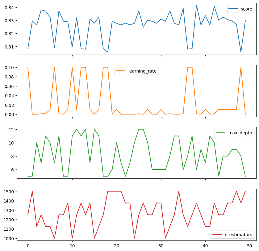
Bayesian Search
- 회차마다 하이퍼 파라미터 값에 대한 조사를 수행할 경우, 사전 지식을 충분히 반영하는 동시에 전체적인 탐색 과정을 체계적으로 수행할 수 있는 방법
- 이전 하이퍼 파라미터 조합의 적용 결과를 기반으로 더 높은 성능 점수를 얻는 하이퍼 파라미터 조합을 예측하는 방식
!pip install optuna

import optuna
from sklearn.model_selection import cross_val_score
from optuna.samplers import TPESampler

optuna.logging.disable_default_handler()
class Objective:
def __init__(self,x_train,y_train,seed):
self.x_train = x_train
self.y_train = y_train
self.seed = seed
num_folds=2
self.cv = KFold(n_splits=num_folds,shuffle=True,random_state=self.seed)
def __call__(self,trial):
hp = {
"max_depth" : trial.suggest_int("max_depth", 2, 5),
"min_samples_split" : trial.suggest_int("min_samples_split", 2, 5),
"criterion" : trial.suggest_categorical("criterion",["gini","entropy"]),
"max_leaf_nodes" : trial.suggest_int("max_leaf_nodes",5,10),
"n_estimators" : trial.suggest_int("n_estimators",10,500,50),
"learning_rate" : trial.suggest_float("learning_rate", 0.01, 0.1),
"verbose": trial.suggest_categorical("verbose",[-1])
}
model = LGBMClassifier(random_state=self.seed,**hp)
scores = cross_val_score(model,self.x_train,self.y_train, cv = self.cv , scoring="roc_auc")
return np.mean(scores)sampler = TPESampler(seed=random_state)
study = optuna.create_study(
direction = "maximize",
sampler = sampler
)
objective = Objective(X_tr, y_tr, random_state)
study.optimize(objective, n_trials=50)
study.best_params
# {'max_depth': 5,
# 'min_samples_split': 3,
# 'criterion': 'entropy',
# 'max_leaf_nodes': 6,
# 'n_estimators': 60,
# 'learning_rate': 0.04480545106871517,
# 'verbose': -1}
study.best_value
# 0.8536850106337968
model = LGBMClassifier(random_state=random_state, **study.best_params)
model.fit(X_tr,y_tr)
pred = model.predict_proba(X_te)[:,1]
roc_auc_score(y_te,pred)
# 0.8988416988416987optuna.visualization.plot_param_importances(study)
'SK네트웍스 Family AI캠프 10기 > Daily 회고' 카테고리의 다른 글
| 24일차. Imbalanced Data & Cross Validation (0) | 2025.02.13 |
|---|---|
| 23일차. Unsupervised Learning (0) | 2025.02.12 |
| 21일차. Supervised Learning - Regression & Classification (0) | 2025.02.10 |
| 20일차. Feature Extraction & Data Encoding (0) | 2025.02.07 |
| 19일차. Machine Learning & Data Preprocessing (0) | 2025.02.07 |


