23일 차 회고.
다른 팀 팀장님께도 토이 프로젝트에서 빠지겠다고 말을 해서 1차 애자일까지만 참여하는 걸로 정해졌다. 이제 주말부터는 개인 공부에 시간을 더 쏟을 예정이다.
1. Unsupervised Learning - Dimensionality Reduction
1-1. 필수 라이브러리 임포트
!pip install --upgrade joblib==1.1.0
!pip install --upgrade scikit-learn==1.1.3
!pip install mglearn

import logging

logging.getLogger('matplotlib.font_manager').setLevel(logging.ERROR)

import mglearn
from sklearn.model_selection import train_test_split

import pandas as pd
import numpy as np

import matplotlib.pyplot as plt
import matplotlib as mpl
import seaborn as sns

%matplotlib inline
1-2. 차원의 저주(The Curse of Dimensionality)
데이터 학습을 위해 차원이 증가하면서 학습 데이터의 수가 차원의 수보다 적어져 성능이 저하된다.
이를 해결하기 위해서는 차원을 축소하거나 데이터를 더 많이 수집해야 한다.
KNN
from sklearn.neighbors import KNeighborsClassifier
from sklearn.preprocessing import OneHotEncoder

X, y = mglearn.datasets.make_forge()
X_tr, X_te, y_tr, y_te = train_test_split(X, y, random_state=0)

X_tr.shape				# (19, 2)

clf = KNeighborsClassifier(n_neighbors=3).fit(X_tr, y_tr)
print(f'훈련용 평가지표: {clf.score(X_tr, y_tr)} / 테스트용 평가지표: {clf.score(X_te, y_te)}')
# 훈련용 평가지표: 0.9473684210526315 / 테스트용 평가지표: 0.8571428571428571

print(f'before: {X.shape}')
enc = OneHotEncoder()
X_enc = enc.fit_transform(X)
print(f'after: {X_enc.shape}')
# before: (26, 2)
# after: (26, 52)

X_tr_enc, X_te_enc, y_tr, y_te = train_test_split(X_enc, y, random_state=0)

X_tr_enc.shape				# (19, 52)

clf = KNeighborsClassifier(n_neighbors=3).fit(X_tr_enc, y_tr)
print(f'훈련용 평가지표: {clf.score(X_tr_enc, y_tr)} / 테스트용 평가지표: {clf.score(X_te_enc, y_te)}')
# 훈련용 평가지표: 0.9473684210526315 / 테스트용 평가지표: 0.42857142857142855 -> overfitting 발생
1-3. 데이터 로드
import pandas as pd
import numpy as np

from sklearn.preprocessing import OneHotEncoder
from sklearn.model_selection import train_test_split
from sklearn.model_selection import cross_val_score
from sklearn.model_selection import KFold

import seaborn as sns

SEED = 42
df = sns.load_dataset('titanic')
y_train = df["survived"]
df = df.drop('survived', axis=1)
# 결측치 미리 채우기
df.age = df.age.fillna(df.age.median())
df.deck = df.deck.fillna(df.deck.mode()[0])
df.embarked = df.embarked.fillna(df.embarked.mode()[0])
df.embark_town = df.embark_town.fillna(df.embark_town.mode()[0])cols = ["age", "fare"]
features = df[cols]
df['new1_age'] = df['age'].map(lambda x: x // 2)
df['new2_age'] = df['age'].map(lambda x: x % 2)
df['new1_fare'] = df['fare'].map(lambda x: x // 2)
df['new2_fare'] = df['fare'].map(lambda x: x % 2)
df.shape # (891, 18)
cols = list(set(df.columns) - set(cols))
enc = OneHotEncoder()
sparse_features = pd.DataFrame(
enc.fit_transform(df[cols]).toarray(),
columns = enc.get_feature_names_out()
)
x_train = pd.concat([features,sparse_features],axis=1)
x_train.shape # (891, 332)
Base Model
model = KNeighborsClassifier(n_neighbors=10)
cv = KFold(n_splits=5,shuffle=True,random_state=SEED)

scores = cross_val_score(model, x_train, y_train, cv = cv , scoring="roc_auc", n_jobs=-1)
base_score = scores.mean()
base_score				# 0.815763031045441
1-4. 주성분 분석(PCA; Principal Component Analysis)
Base Model
sparse_features.shape[1] # 330from sklearn.decomposition import PCA
pca = PCA(n_components=sparse_features.shape[1], random_state=SEED)
# 주성분 학습
pca.fit(sparse_features)
sum(pca.explained_variance_ratio_) # 압축 정도: 0.9999999999999997
# 주성분 예측
tmp = pd.DataFrame(pca.transform(sparse_features)).add_prefix("pca_")
x_train = pd.concat([features, tmp], axis=1) # feature: 수치형 데이터 / tmp: 범주형 데이터 -> 차원 축소
print(f'after: {x_train.shape}') # after: (891, 332)
model = KNeighborsClassifier(n_neighbors=10)
scores = cross_val_score(model, x_train, y_train, cv = cv, scoring="roc_auc", n_jobs=-1)
print(f'score: {scores.mean()} / base_score: {base_score}')
# score: 0.8158991780842427 / base_score: 0.815763031045441
n_components = 2
pca2 = PCA(n_components=2, random_state=SEED)
pca2.fit(sparse_features)
sum(pca2.explained_variance_ratio_)		# 0.30258569160962595

tmp = pd.DataFrame(pca2.transform(sparse_features)).add_prefix("pca_")
x_train = pd.concat([features, tmp], axis=1)
print(f'after: {x_train.shape}')		# after: (891, 4)

model = KNeighborsClassifier(n_neighbors=10)
scores = cross_val_score(model, x_train, y_train, cv = cv, scoring="roc_auc", n_jobs=-1)
print(f'score: {scores.mean()} / base_score: {base_score}')
# score: 0.797416401065853 / base_score: 0.815763031045441
n_components = 15
pca15 = PCA(n_components=15, random_state=SEED)
pca15.fit(sparse_features)
sum(pca15.explained_variance_ratio_)		# 0.7362243873745266

tmp = pd.DataFrame(pca15.transform(sparse_features)).add_prefix("pca_")
x_train = pd.concat([features, tmp], axis=1)
print(f'after: {x_train.shape}')		# after: (891, 17)

model = KNeighborsClassifier(n_neighbors=10)
scores = cross_val_score(model, x_train, y_train, cv = cv, scoring="roc_auc", n_jobs=-1)
print(f'score: {scores.mean()} / base_score: {base_score}')
# score: 0.8257991549587771 / base_score: 0.815763031045441
1-5. 특이값 분해(SVD; Singular Value Decomposition)
특이값 분해는 임의의 m × n 차원의 행렬 A에 대하여 다음과 같이 행렬을 분해하는 방법이다.
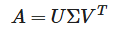
특이값 분해는 음성 데이터와 같은 복원이 필요한 데이터를 분석할 때 주로 사용한다.
특이값 분해 및 복원
np.random.seed(121)
a = np.random.randn(4,4)
np.round(a,3)
# array([[-0.212, -0.285, -0.574, -0.44 ],
#        [-0.33 ,  1.184,  1.615,  0.367],
#        [-0.014,  0.63 ,  1.71 , -1.327],
#        [ 0.402, -0.191,  1.404, -1.969]])
from numpy.linalg import svd
# 특이값 분해
U, Sigma, Vt = svd(a)
print(U.shape, Sigma.shape, Vt.shape) # (4, 4) (4,) (4, )
print('U matrix:\n',np.round(U, 3))
# U matrix:
# [[-0.079 -0.318 0.867 0.376]
# [ 0.383 0.787 0.12 0.469]
# [ 0.656 0.022 0.357 -0.664]
# [ 0.645 -0.529 -0.328 0.444]]
print('Sigma Value:\n',np.round(Sigma, 3))
# Sigma Value:
# [3.423 2.023 0.463 0.079]
print('V transpose matrix:\n',np.round(Vt, 3))
# V transpose matrix:
# [[ 0.041 0.224 0.786 -0.574]
# [-0.2 0.562 0.37 0.712]
# [-0.778 0.395 -0.333 -0.357]
# [-0.593 -0.692 0.366 0.189]]# Sigma를 0을 포함한 대칭행렬로 변환
Sigma_mat = np.diag(Sigma)
# 복원
a_ = np.dot(np.dot(U, Sigma_mat), Vt)
print(f'원본: {np.round(a,3)}')
print('-'*40)
print(f'복원: {np.round(a_, 3)}')
# 원본: [[-0.212 -0.285 -0.574 -0.44 ]
# [-0.33 1.184 1.615 0.367]
# [-0.014 0.63 1.71 -1.327]
# [ 0.402 -0.191 1.404 -1.969]]
# ----------------------------------------
# 복원: [[-0.212 -0.285 -0.574 -0.44 ]
# [-0.33 1.184 1.615 0.367]
# [-0.014 0.63 1.71 -1.327]
# [ 0.402 -0.191 1.404 -1.969]]
Base Model
from sklearn.decomposition import TruncatedSVD

svd = TruncatedSVD(n_components=sparse_features.shape[1], random_state=SEED)
svd.fit(sparse_features)
sum(svd.explained_variance_ratio_)		# 0.9999999999999979

tmp = pd.DataFrame(svd.transform(sparse_features)).add_prefix("svd_")
x_train = pd.concat([features, tmp], axis=1)
print(f'after: {x_train.shape}')		# after: (891, 332)

model = KNeighborsClassifier(n_neighbors=10)
base_score = cross_val_score(model, x_train, y_train, cv = cv, scoring="roc_auc", n_jobs=-1).mean()
print(f'base_score: {base_score}')		# base_score: 0.8160958779824352
n_components = 2
svd2 = TruncatedSVD(n_components=2, random_state=SEED)
svd2.fit(sparse_features)
sum(svd2.explained_variance_ratio_)		# 0.21212890511257992

tmp = pd.DataFrame(svd2.transform(sparse_features)).add_prefix("svd_")
x_train = pd.concat([features, tmp], axis=1)
print(f'after: {x_train.shape}')		# after: (891, 4)

model = KNeighborsClassifier(n_neighbors=10)
scores = cross_val_score(model, x_train, y_train, cv = cv, scoring="roc_auc", n_jobs=-1)
print(f'score: {scores.mean()} / base_score: {base_score}')
# score: 0.7958265580897994 / base_score: 0.8160958779824352
n_components = 15
svd15 = TruncatedSVD(n_components=15, random_state=SEED)
svd15.fit(sparse_features)
sum(svd15.explained_variance_ratio_)		# 0.7264584746122391

tmp = pd.DataFrame(svd15.transform(sparse_features)).add_prefix("svd_")
x_train = pd.concat([features, tmp], axis=1)
print(f'after: {x_train.shape}')		# after: (891, 17)

model = KNeighborsClassifier(n_neighbors=10)
scores = cross_val_score(model, x_train, y_train, cv = cv, scoring="roc_auc", n_jobs=-1)
print(f'score: {scores.mean()} / base_score: {base_score}')
# score: 0.8260096949480781 / base_score: 0.8160958779824352
1-6. 비음수 행렬 분해(NMF; Non-negative Matrix Factorization)
비음수 행렬 분해는 음수를 포함하지 않는 행렬 X를 음수를 포함하지 않는 행렬 W와 H의 곱으로 분해하는 방법이다.
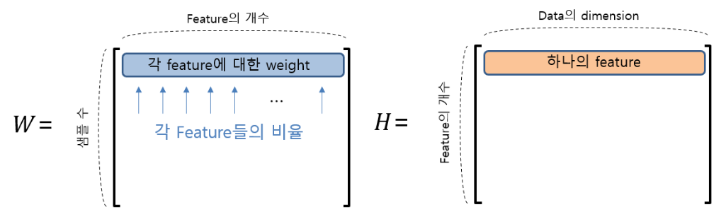
비음수 행렬 분해는 추천 시스템을 구현할 때 주로 사용한다.
Base Model
from sklearn.decomposition import NMF

nmf = NMF(n_components=sparse_features.shape[1], random_state=SEED, max_iter=500)
nmf.fit(sparse_features)

(nmf.components_ < 0).sum()			# 0
nmf.components_.shape				# (330, 330)

tmp = pd.DataFrame(nmf.transform(sparse_features)).add_prefix("nmf_")
x_train = pd.concat([features, tmp], axis=1)
print(f'after: {x_train.shape}')		# after: (891, 332)

model = KNeighborsClassifier(n_neighbors=10)
base_score = cross_val_score(model, x_train, y_train, cv = cv, scoring="roc_auc", n_jobs=-1).mean()
print(f'base_score: {base_score}')		# base_score: 0.7313518836299018
n_component = 5
nmf5 = NMF(n_components=5, random_state=SEED, max_iter=500)
nmf5.fit(sparse_features)

(nmf5.components_ < 0).sum()			# 0
nmf5.components_.shape				# (5, 330)

tmp = pd.DataFrame(nmf5.transform(sparse_features)).add_prefix("nmf_")
x_train = pd.concat([features, tmp], axis=1)
print(f'after: {x_train.shape}')		# after: (891, 7)

model = KNeighborsClassifier(n_neighbors=10)
scores = cross_val_score(model, x_train, y_train, cv = cv, scoring="roc_auc", n_jobs=-1)
print(f'score: {scores.mean()} / base_score: {base_score}')
# score: 0.7199486147184602 / base_score: 0.7313518836299018
n_component = 50
nmf50 = NMF(n_components=50, random_state=SEED, max_iter=500)
nmf50.fit(sparse_features)

(nmf50.components_ < 0).sum()			# 0
nmf50.components_.shape				# (50, 330)

tmp = pd.DataFrame(nmf50.transform(sparse_features)).add_prefix("nmf_")
x_train = pd.concat([features, tmp], axis=1)
print(f'after: {x_train.shape}')		# after: (891, 52)

model = KNeighborsClassifier(n_neighbors=10)
scores = cross_val_score(model, x_train, y_train, cv = cv, scoring="roc_auc", n_jobs=-1)
print(f'score: {scores.mean()} / base_score: {base_score}')
# score: 0.7227777788480636 / base_score: 0.7313518836299018
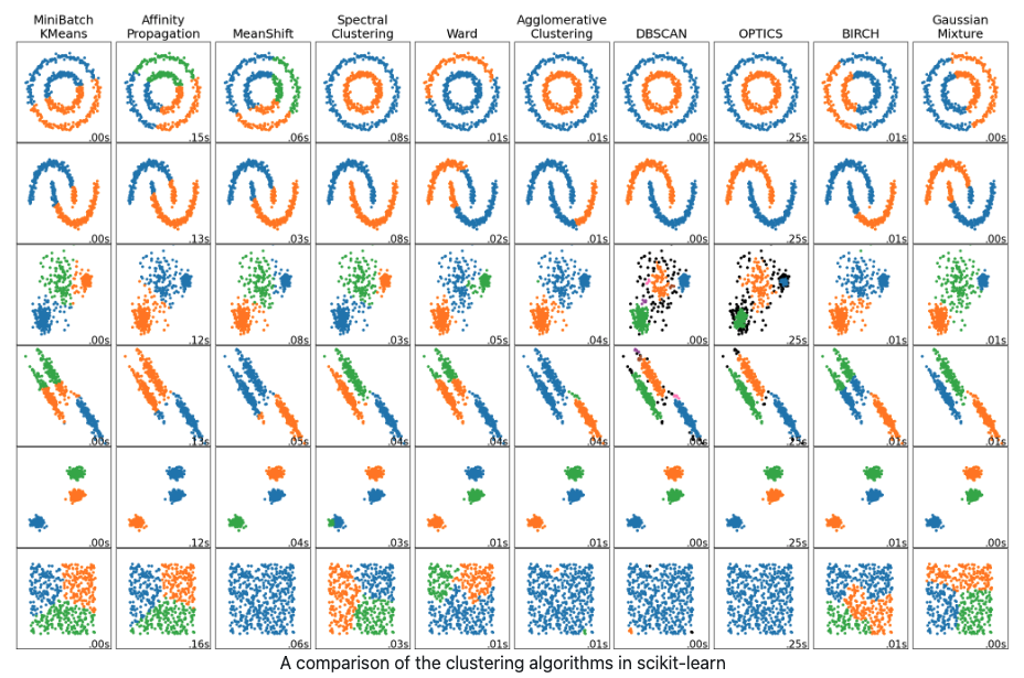
2. Unsupervised Learning - Clustering
2-1. 필수 라이브러리 임포트
!pip install --upgrade joblib==1.1.0
!pip install --upgrade scikit-learn==1.1.3
!pip install mglearn

import logging

logging.getLogger('matplotlib.font_manager').setLevel(logging.ERROR)

import mglearn
from sklearn.model_selection import train_test_split

import pandas as pd
import numpy as np

import matplotlib.pyplot as plt
import matplotlib as mpl
import seaborn as sns

%matplotlib inline
2-2. Clustering
Clustering은 Unsupervised Learning로 label(정답)이 존재하지 않는 상태에서 학습을 통해 비슷한 개체끼리 그룹으로 묶는다.
2-3. K-means
K-means
- K개의 랜덤한 중심점으로부터 가까운 데이터들을 묶는 군집화 기법
- 평균을 사용하기 때문에 이상치에 민감하다.
- 거리를 재기 때문에 Scaling이 필수다.
알고리즘 작동 방식
- Initialization: 랜덤으로 중심을 초기화한다.
- Assign Points: 데이터 포인트를 가장 가까운 cluster 중심으로 할당한다.
- Recompute Centers: cluster에 할당된 데이터 포인트의 평균으로 cluster 중심을 재정의한다.
- 포인트에 변화가 없을 때까지 앞의 과정을 반복한다.

모델학습
from sklearn.datasets import make_blobs

X, y = make_blobs(random_state=1)
X.shape, y.shape				((100, 2), (100,))
from sklearn.cluster import KMeans
kmeans = KMeans(n_clusters=3)
# Unsupervised Learning -> features만 학습
kmeans.fit(X)# label -> target
kmeans.labels_
# array([1, 0, 0, 0, 2, 2, 2, 0, 1, 1, 0, 0, 2, 1, 2, 2, 2, 1, 0, 0, 2, 0,
# 2, 1, 0, 2, 2, 1, 1, 2, 1, 1, 2, 1, 0, 2, 0, 0, 0, 2, 2, 0, 1, 0,
# 0, 2, 1, 1, 1, 1, 0, 2, 2, 2, 1, 2, 0, 0, 1, 1, 0, 2, 2, 0, 0, 2,
# 1, 2, 1, 0, 0, 0, 2, 1, 1, 0, 2, 2, 1, 0, 1, 0, 0, 2, 1, 1, 1, 1,
# 0, 1, 2, 1, 1, 0, 0, 2, 2, 1, 2, 1], dtype=int32)kmeans.predict(X)
# array([1, 0, 0, 0, 2, 2, 2, 0, 1, 1, 0, 0, 2, 1, 2, 2, 2, 1, 0, 0, 2, 0,
# 2, 1, 0, 2, 2, 1, 1, 2, 1, 1, 2, 1, 0, 2, 0, 0, 0, 2, 2, 0, 1, 0,
# 0, 2, 1, 1, 1, 1, 0, 2, 2, 2, 1, 2, 0, 0, 1, 1, 0, 2, 2, 0, 0, 2,
# 1, 2, 1, 0, 0, 0, 2, 1, 1, 0, 2, 2, 1, 0, 1, 0, 0, 2, 1, 1, 1, 1,
# 0, 1, 2, 1, 1, 0, 0, 2, 2, 1, 2, 1], dtype=int32)y
# array([0, 1, 1, 1, 2, 2, 2, 1, 0, 0, 1, 1, 2, 0, 2, 2, 2, 0, 1, 1, 2, 1,
# 2, 0, 1, 2, 2, 0, 0, 2, 0, 0, 2, 0, 1, 2, 1, 1, 1, 2, 2, 1, 0, 1,
# 1, 2, 0, 0, 0, 0, 1, 2, 2, 2, 0, 2, 1, 1, 0, 0, 1, 2, 2, 1, 1, 2,
# 0, 2, 0, 1, 1, 1, 2, 0, 0, 1, 2, 2, 0, 1, 0, 1, 1, 2, 0, 0, 0, 0,
# 1, 0, 2, 0, 0, 1, 1, 2, 2, 0, 2, 0])
모델 결과 분석
mglearn.discrete_scatter(X[:,0], X[:,1], kmeans.labels_, markers='o')
mglearn.discrete_scatter(
    kmeans.cluster_centers_[:,0], kmeans.cluster_centers_[:,1],
    [0,1,2], markers='v', markeredgewidth=2
)
fig, axes = plt.subplots(1, 2, figsize=(10,5))

# n_clusters = 2
kmeans = KMeans(n_clusters=2)
kmeans.fit(X)
mglearn.discrete_scatter(X[:,0], X[:,1], kmeans.labels_, ax=axes[0])

# n_clusters = 5
kmeans = KMeans(n_clusters=5)
kmeans.fit(X)
mglearn.discrete_scatter(X[:,0], X[:,1], kmeans.labels_, ax=axes[1])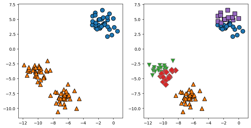
K-means 실패 이유
- 각 cluster를 정의하는 것이 중심 하나뿐이기 때문에, cluster는 둥근 형태이면서 데이터가 밀집되어 있어야 한다.
- cluster의 개수(n_clusters)의 초기값을 미리 알 수 없기 때문에 사용에 유의해야 한다.
x_data, y_data = make_blobs(n_samples=200, cluster_std=[1.0, 2.5, 0.5], random_state=170)
kmeans = KMeans(n_clusters=3, random_state=0).fit(x_data)

mglearn.discrete_scatter(x_data[:,0], x_data[:,1], kmeans.labels_)

plt.legend(["Clustering 0", "Clustering 1", "Clustering 2"], loc='best')

plt.xlabel('feature 0')
plt.ylabel('feature 1')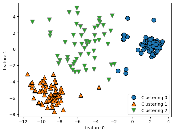
x_data, y_data = make_blobs(random_state=170, n_samples=600)

rng = np.random.RandomState(74)
transformation = rng.normal(size=(2, 2))
x_data = np.dot(x_data, transformation)

kmeans = KMeans(n_clusters=3).fit(x_data)

mglearn.discrete_scatter(x_data[:,0], x_data[:,1], kmeans.labels_, markers='o')
mglearn.discrete_scatter(
    kmeans.cluster_centers_[:,0], kmeans.cluster_centers_[:,1],
    [0,1,2], markers='v', markeredgewidth=2
)

plt.legend(["Clustering 0", "Clustering 1", "Clustering 2"], loc='best')

plt.xlabel('feature 0')
plt.ylabel('feature 1')
2-4. 군집 타당성 평가
군집 타당성 평가
- Clustering은 정답이 없기 때문에, Supervised Learning에서 사용하는 Accuracy 등의 지표로 평가할 수 없다.
- 군집 타당성 지표를 통해 군집을 만든 결과가 얼마나 유용한지 따진다.
- 군집 간 분산(Inter-Cluster Variance) 최대화
- 군집 내 분산(Inner-Cluster Variance) 최소화
데이터 로드
SEED = 42from sklearn.datasets import load_digits
digits = load_digits()
digits.data[0].reshape(8, 8)
# array([[ 0., 0., 5., 13., 9., 1., 0., 0.],
# [ 0., 0., 13., 15., 10., 15., 5., 0.],
# [ 0., 3., 15., 2., 0., 11., 8., 0.],
# [ 0., 4., 12., 0., 0., 8., 8., 0.],
# [ 0., 5., 8., 0., 0., 9., 8., 0.],
# [ 0., 4., 11., 0., 1., 12., 7., 0.],
# [ 0., 2., 14., 5., 10., 12., 0., 0.],
# [ 0., 0., 6., 13., 10., 0., 0., 0.]])x = digits.data / 255 # Min Max Scaling
y = digits.target
x.shape, y.shape # ((1797, 64), (1797,))
np.random.seed(SEED)
idx = np.arange(x.shape[0])
np.random.shuffle(idx)
x = x[idx]
y = y[idx]
x.shape, y.shape # ((1797, 64), (1797,))np.random.seed(SEED)
idx = np.arange(x.shape[0])
np.random.shuffle(idx)
# 랜덤하게 변경된 index값에 맞는 x, y 데이터 순서 변경
x = x[idx]
y = y[idx]
kmeans = KMeans(n_clusters=10, random_state=SEED)
kmeans.fit(x)
사전에 정의된 그룹이 있는 경우
- homogeneity
- 각 군집이 동일한 클래스로 구성되어 있는 정도
from sklearn.metrics import homogeneity_score

homogeneity_score(y,kmeans.labels_)
# 0.737996379571194- completeness
- 각 클래스에 대하여 동일한 군집으로 구성되어 있는 정도
from sklearn.metrics import completeness_score

completeness_score(y,kmeans.labels_)
# 0.74602699054445- v-measure
- homogeneity와 completeness의 조화 평균
from sklearn.metrics import v_measure_score

v_measure_score(y, kmeans.labels_)
# 0.7419899567232477
사전에 정의된 그룹이 없는 경우
- silhouette coefficient(실루엣 계수)
- 밀집된 클러스터에는 좋지만 모양이 복잡할 때는 평가가 잘 들어맞지 않는다.
- -1 ~ 1의 값을 가진다.
- 1에 가까울수록, 명확하게 군집화됨을 의미한다.
- 0에 가까울수록, 군집 간의 거리가 가까워진다는 것을 의미한다.
- 음수일 경우, 잘못된 방식으로 군집화되었다는 것을 의미한다.
from sklearn.metrics import silhouette_score

silhouette_score(x, kmeans.labels_)
# 0.18226082805532845
2-5. Clustering Methods
def print_score(x,y,pred):
    print(f"homogeneity: {homogeneity_score(y,pred)}")
    print(f"completeness: {completeness_score(y,pred)}")
    print(f"v_measure: {v_measure_score(y,pred)}")
    print('-'*50)
    print(f"silhouette: {silhouette_score(x,pred)}")
Mini Batch KMeans
from sklearn.cluster import MiniBatchKMeans

kmeans = MiniBatchKMeans(n_clusters=10,random_state=SEED,batch_size=512 ).fit(x)
print_score(x,y,kmeans.labels_)
# homogeneity: 0.7129288903522629
# completeness: 0.7288991277425318
# v_measure: 0.720825562825275
# ----------------------------------------
# silhouette: 0.18472538252636414
Agglomerative Clustering
- 지정된 개수의 cluster가 남을 때까지 비슷한 cluster를 합치는 알고리즘
mglearn.plots.plot_agglomerative_algorithm()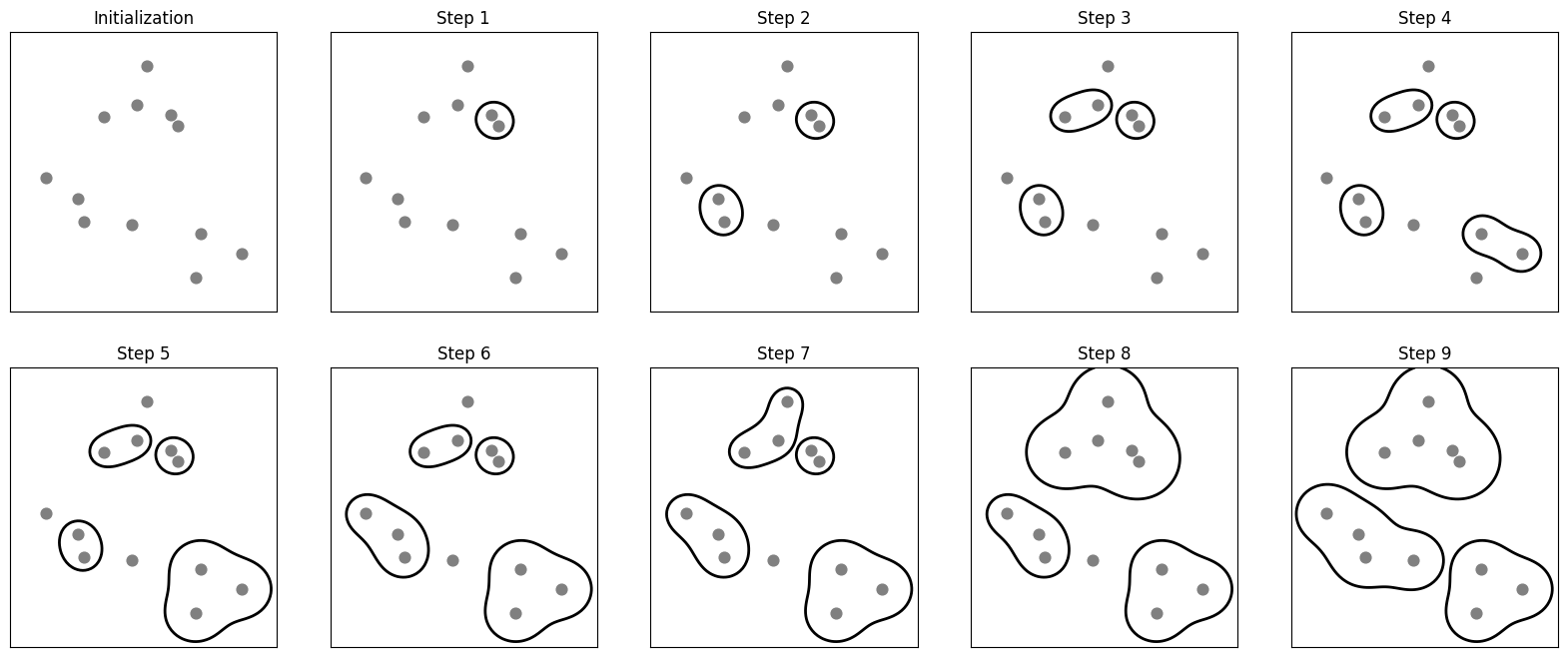
from sklearn.cluster import AgglomerativeClustering

ac = AgglomerativeClustering(n_clusters=10).fit(x)
print_score(x,y,ac.labels_)
# homogeneity: 0.8575128719504722
# completeness: 0.8790955851724198
# v_measure: 0.8681701126909083
# ----------------------------------------
# silhouette: 0.17849659940596496
DBSCAN
- cluster의 개수를 미리 지정할 필요가 없다.
- 데이터 샘플들이 몰려있는 지점을 찾아 묶어서 군집화한다.
mglearn.plots.plot_dbscan()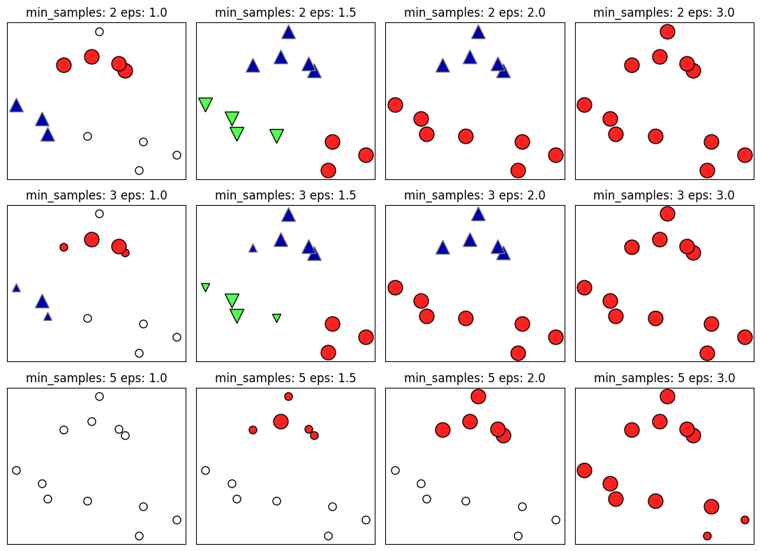
from sklearn.cluster import DBSCAN

dbscan = DBSCAN(min_samples=3,eps=0.05,n_jobs=-1).fit(x)
print_score(x,y,dbscan.labels_)
# homogeneity: 0.07120590002352155
# completeness: 0.3582655753349777
# v_measure: 0.11880007964616035
# ----------------------------------------
# silhouette: -0.29235730958906886
3. Overfitting & Underfitting
3-1. Overfitting & Underfitting
과대적합(Overfitting)
- Overfitting은 모델이 학습 데이터에 필요 이상으로 적합한 것을 말한다.
- 데이터 내의 존재하는 규칙뿐만이 아니라 불완전한 샘플도 학습한다.
과소적합(Underfitting)
- Underfitting은 모델이 학습 데이터에 제대로 적합하지 못한 것을 말한다.
- 데이터 내에 존재하는 규칙도 제대로 학습하지 못한 상태이다.
'SK네트웍스 Family AI캠프 10기 > Daily 회고' 카테고리의 다른 글
| 25일차. AutoML & XAI & Pipeline (0) | 2025.02.14 |
|---|---|
| 24일차. Imbalanced Data & Cross Validation (0) | 2025.02.13 |
| 22일차. Supervised Learning - Classification & Ensemble & HPO (0) | 2025.02.11 |
| 21일차. Supervised Learning - Regression & Classification (0) | 2025.02.10 |
| 20일차. Feature Extraction & Data Encoding (0) | 2025.02.07 |


