더보기
24일 차 회고.
이제 곧 토이 프로젝트 팀에서 나가게 될 텐데 내가 무엇을 해야 할지 무엇에 집중해야 할지 정리해봐야 할 것 같다.
1. Imbalanced Data
1-1. Imbalanced Data
불균형 데이터는 목표 변수(Target)가 범주형 데이터일 경우, 범주별로 관측치의 개수, 비율의 차이가 많이 나는 데이터를 말한다.
불균형 데이터를 이용한 모델링 문제점
- 소수 집단(Minority Class)의 관측치 개수가 적을 경우, 소수 집단의 모집단 분포를 샘플링한 소수의 관측치가 소수 집단을 대표하기에는 부족하기 때문에 분류 모델이 overfitting에 빠질 위험이 있다.
- 정상(Majority Class) : 비정상(Minority Class)의 비율이 99 : 1이라고 할 경우, 모델이 정상만 학습을 하여도 정확도가 99%가 되기 때문에 비정상을 제대로 분류하지 못하는 모델이 될 수 있다.
불균형 데이터 처리 방법
- 평가 기준 변경
- Confusion Matrix
- 예측 결과를 테이블 형태로 보여준다.
- Precision
- Positive 클래스에 속한다고 출력한 샘플 중 실제로 Positive 클래스에 속하는 샘플 수의 비율
- Recall
- 실제 Positive 클래스에 속한 샘플 중 Positive 클래스에 속한다고 출력한 샘플 수의 비율
- F1 Score
- Precision과 Recall의 가중 조화 평균
- Threshold 값 조절 필수
- ROC Curves
- 클래스 판별 기준 값의 변화에 따른 Fall-out과 Recall의 변화를 시각화해 준다.
- Confusion Matrix
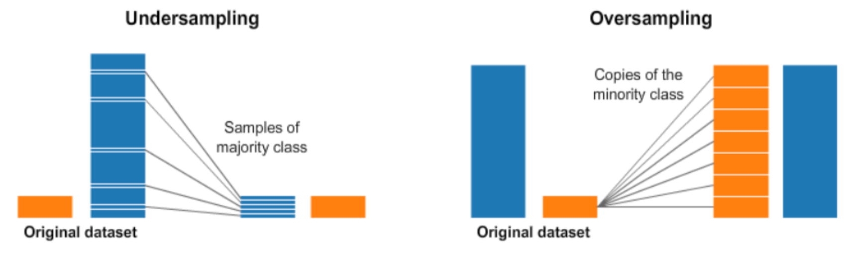
- Resampling
- Under-Sampling
- Over-Sampling
- overfitting 될 확률이 높다.
1-2. 예제
from sklearn.datasets import make_classification
from sklearn.linear_model import LogisticRegression
from sklearn.dummy import DummyClassifier

from sklearn.model_selection import train_test_split

from sklearn.metrics import roc_curve
from sklearn.metrics import roc_auc_score
from sklearn.metrics import precision_recall_curve
from sklearn.metrics import auc

import numpy as np
import pandas as pd

np.set_printoptions(formatter={'float_kind': lambda x: "{0:0.6f}".format(x)})

import logging

logging.getLogger('matplotlib.font_manager').setLevel(logging.ERROR)
import matplotlib.pyplot as plt
import matplotlib as mpl
import seaborn as sns
%matplotlib inline
mpl.rc('axes', unicode_minus=False)def plot_roc_curve(test_y, naive_probs, model_probs,clf_name):
fpr, tpr, _ = roc_curve(test_y, naive_probs)
plt.plot(fpr, tpr, linestyle='--', label='No Skill')
fpr, tpr, _ = roc_curve(test_y, model_probs)
plt.plot(fpr, tpr, marker='.', label=clf_name)
plt.xlabel('False Positive Rate')
plt.ylabel('True Positive Rate')
plt.legend()
plt.show()# 99:1 비율로 unbalanced data 생성
X, y = make_classification(n_samples=1000, n_classes=2, weights=[0.99, 0.01], random_state=1)
X.shape, y.shape, np.unique(y)trainX, testX, trainy, testy = train_test_split(X, y, test_size=0.5, random_state=2, stratify=y)
trainX.shape, testX.shape, trainy.shape, testy.shape
# ((500, 20), (500, 20), (500,), (500,))print('Dataset: Class0=%d, Class1=%d' % (len(y[y==0]), len(y[y==1])))
print('Train: Class0=%d, Class1=%d' % (len(trainy[trainy==0]), len(trainy[trainy==1])))
print('Test: Class0=%d, Class1=%d' % (len(testy[testy==0]), len(testy[testy==1])))
# Dataset: Class0=985, Class1=15
# Train: Class0=492, Class1=8
# Test: Class0=493, Class1=7
ROC-AUC Curve
# Dummy Model
model = DummyClassifier(strategy='stratified')
model.fit(trainX, trainy)
yhat = model.predict_proba(testX)
print(yhat[0:5])

naive_probs = yhat[:, 1]

dummy_roc_auc = roc_auc_score(testy, naive_probs)
print('No Skill ROC AUC %.3f' % dummy_roc_auc)

# [[1.000000 0.000000]
#  [1.000000 0.000000]
#  [1.000000 0.000000]
#  [1.000000 0.000000]
#  [1.000000 0.000000]]
# No Skill ROC AUC 0.494
# Logistic Regression
model = LogisticRegression(solver='lbfgs')
model.fit(trainX, trainy)
yhat = model.predict_proba(testX)
print(yhat[0:5])
model_probs = yhat[:, 1]
model_roc_auc = roc_auc_score(testy, model_probs)
print('Logistic ROC AUC %.3f' % model_roc_auc)
# [[0.958213 0.041787]
# [0.998591 0.001409]
# [0.993148 0.006852]
# [0.971451 0.028549]
# [0.999532 0.000468]]
# Logistic ROC AUC 0.869plot_roc_curve(testy, naive_probs, model_probs, clf_name='Logistic')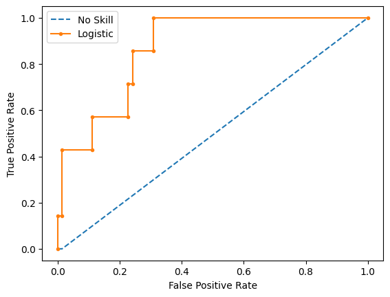
Precision-Recall Curve
def plot_pr_curve(test_y, model_probs,clf_name):
    no_skill = len(test_y[test_y==1]) / len(test_y)

	plt.plot([0, 1], [no_skill, no_skill], linestyle='--', label='No Skill')

	precision, recall, _ = precision_recall_curve(testy, model_probs)
    plt.plot(recall, precision, marker='.', label=clf_name)

	plt.xlabel('Recall')
    plt.ylabel('Precision')

	plt.legend()

	plt.show()
# Dummy Model
model = DummyClassifier(strategy='stratified')
model.fit(trainX, trainy)
yhat = model.predict_proba(testX)
print(yhat[0:5])
naive_probs = yhat[:, 1]
precision, recall, _ = precision_recall_curve(testy, naive_probs)
dummy_auc_score = auc(recall, precision)
print('No Skill PR AUC: %.3f' % dummy_auc_score)
# [[1.000000 0.000000]
# [1.000000 0.000000]
# [1.000000 0.000000]
# [1.000000 0.000000]
# [1.000000 0.000000]]
# No Skill PR AUC: 0.007# Logistic Regression
model = LogisticRegression(solver='lbfgs')
model.fit(trainX, trainy)
yhat = model.predict_proba(testX)
print(yhat[0:5])
model_probs = yhat[:, 1]
precision, recall, _ = precision_recall_curve(testy, model_probs)
model_auc_score = auc(recall, precision)
print('Logistic PR AUC: %.3f' % model_auc_score)
# [[0.958213 0.041787]
# [0.998591 0.001409]
# [0.993148 0.006852]
# [0.971451 0.028549]
# [0.999532 0.000468]]
# Logistic PR AUC: 0.231plot_pr_curve(testy, model_probs,clf_name='Logistic')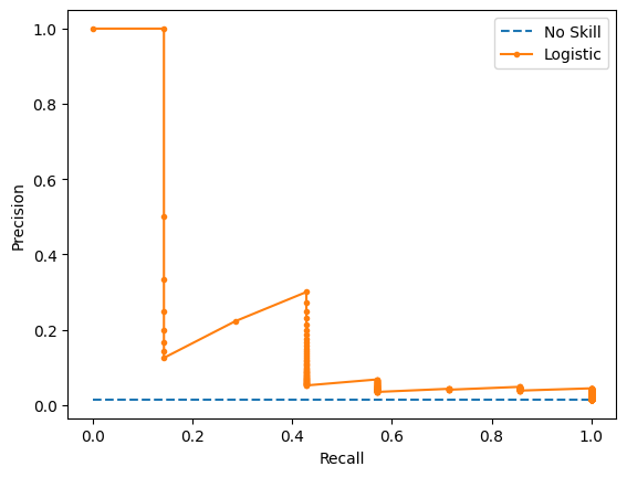
해석
print(f'No Skill ROC AUC: {dummy_roc_auc} / Logistic ROC AUC: {model_roc_auc}')
print('=============================================================================')
print(f'No Skill PR AUC: {dummy_auc_score} / Logistic PR AUC: {model_auc_score}')

# No Skill ROC AUC: 0.49391480730223125 / Logistic ROC AUC: 0.8690234714575485
# =============================================================================
# No Skill PR AUC: 0.007 / Logistic PR AUC: 0.23117895823734802
Resampling
from sklearn.datasets import *
from sklearn.model_selection import train_test_split
from sklearn.metrics import recall_score
from sklearn.svm import SVC

import scipy as sp
def classification_result(n0, n1, title=""):
rv1 = sp.stats.multivariate_normal([-1, 0], [[1, 0], [0, 1]])
rv2 = sp.stats.multivariate_normal([+1, 0], [[1, 0], [0, 1]])
X0 = rv1.rvs(n0, random_state=0)
X1 = rv2.rvs(n1, random_state=0)
X = np.vstack([X0, X1])
y = np.hstack([np.zeros(n0), np.ones(n1)])
x1min = -4; x1max = 4
x2min = -2; x2max = 2
xx1 = np.linspace(x1min, x1max, 1000)
xx2 = np.linspace(x2min, x2max, 1000)
X1, X2 = np.meshgrid(xx1, xx2)
plt.contour(X1, X2, rv1.pdf(np.dstack([X1, X2])), levels=[0.05], linestyles="dashed")
plt.contour(X1, X2, rv2.pdf(np.dstack([X1, X2])), levels=[0.05], linestyles="dashed")
model = SVC(kernel="linear", C=1e4, random_state=0).fit(X, y)
Y = np.reshape(model.predict(np.array([X1.ravel(), X2.ravel()]).T), X1.shape)
plt.scatter(X[y == 0, 0], X[y == 0, 1], marker='x', label="0 클래스")
plt.scatter(X[y == 1, 0], X[y == 1, 1], marker='o', label="1 클래스")
plt.contour(X1, X2, Y, colors='k', levels=[0.5])
y_pred = model.predict(X)
plt.xlim(-4, 4)
plt.ylim(-3, 3)
plt.xlabel("x1")
plt.ylabel("x2")
plt.title(title)
return model, X, y, y_pred
plt.subplot(121)
model1, X1, y1, y_pred1 = classification_result(200, 200, "Balanced Data (5:5)")
plt.subplot(122)
model2, X2, y2, y_pred2 = classification_result(200, 20, "Imbalanced Data (9:1)")
plt.tight_layout()
plt.show();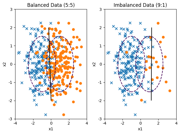
from sklearn.metrics import classification_report, confusion_matrix

print(classification_report(y1, y_pred1))
print('=======================================================')
print(classification_report(y2, y_pred2))

#               precision    recall  f1-score   support
#
#          0.0       0.86      0.83      0.84       200
#          1.0       0.84      0.86      0.85       200
#
#     accuracy                           0.85       400
#    macro avg       0.85      0.85      0.85       400
# weighted avg       0.85      0.85      0.85       400
#
# =======================================================
#               precision    recall  f1-score   support
#
#          0.0       0.96      0.98      0.97       200
#          1.0       0.75      0.60      0.67        20
#
#     accuracy                           0.95       220
#    macro avg       0.86      0.79      0.82       220
# weighted avg 0.94 0.95 0.94 220- imbalanced-learn 패키지
# !pip install imbalanced-learn

def classification_result2(X, y, title=""):
    plt.contour(X1, X2, rv1.pdf(np.dstack([X1, X2])), levels=[0.05], linestyles="dashed")
    plt.contour(X1, X2, rv2.pdf(np.dstack([X1, X2])), levels=[0.05], linestyles="dashed")
    model = SVC(kernel="linear", C=1e4, random_state=0).fit(X, y)
    Y = np.reshape(model.predict(np.array([X1.ravel(), X2.ravel()]).T), X1.shape)
    plt.scatter(X[y == 0, 0], X[y == 0, 1], marker='x', label="0 클래스")
    plt.scatter(X[y == 1, 0], X[y == 1, 1], marker='o', label="1 클래스")
    plt.contour(X1, X2, Y, colors='k', levels=[0.5])
    y_pred = model.predict(X)
    plt.xlim(-4, 4)
    plt.ylim(-3, 3)
    plt.xlabel("x1")
    plt.ylabel("x2")
    plt.title(title)
    return model

n0 = 200; n1 = 20
rv1 = sp.stats.multivariate_normal([-1, 0], [[1, 0], [0, 1]])
rv2 = sp.stats.multivariate_normal([+1, 0], [[1, 0], [0, 1]])
X0 = rv1.rvs(n0, random_state=0)
X1 = rv2.rvs(n1, random_state=0)
X_imb = np.vstack([X0, X1])
y_imb = np.hstack([np.zeros(n0), np.ones(n1)])

x1min = -4; x1max = 4
x2min = -2; x2max = 2
xx1 = np.linspace(x1min, x1max, 1000)
xx2 = np.linspace(x2min, x2max, 1000)
X1, X2 = np.meshgrid(xx1, xx2)
Under-Sampling
- Random Under Sampler
- 무작위로 데이터를 없애는 단순 샘플링 방법
from imblearn.under_sampling import RandomUnderSampler

X_samp, y_samp = RandomUnderSampler(random_state=0).fit_resample(X_imb, y_imb)

plt.subplot(121)
classification_result2(X_imb, y_imb)
plt.subplot(122)
model_samp = classification_result2(X_samp, y_samp)
print(classification_report(y_imb, model_samp.predict(X_imb)))
#               precision    recall  f1-score   support
#
#          0.0       0.99      0.92      0.95       200
#          1.0       0.51      0.90      0.65        20
#
#     accuracy                           0.91       220
#    macro avg       0.75      0.91      0.80       220
# weighted avg 0.95 0.91 0.92 220- One Sided Selection
- 토멕 링크(Tomek Links)
- 서로 다른 클래스에 속해있지만 가장 가까이 붙어있는 한 쌍의 데이터
- 토멕 링크를 가진 데이터 쌍들 중 다수의 클래스에 속해있는 데이터를 삭제해서 under sampling을 수행한다.
- CNN(Condensed Nearest Neighbour)
- 다수 클래스에 밀접한 데이터가 없을 때까지 데이터를 제거하여 데이터 분포에서 대표적인 데이터만 남도록 한다.
- 다수 클래스의 데이터 포인트와 가장 가까운 데이터가 소수 클래스인 다수 클래스 데이터 외에는 모두 삭제하는 방법
- OSS(One-Side Selection)
- Tomek Links와 CNN을 같이 수행하는 방법
- Tomek Links로 분류 경계에 존재하는 데이터들을 under sampling하는 동시에, CNN으로 다수 클래스가 밀집한 데이터가 없을 때까지 데이터를 제거하여 분포에서 대표적인 데이터만 남게 한다.
- 토멕 링크(Tomek Links)
from imblearn.under_sampling import OneSidedSelection

X_samp, y_samp = OneSidedSelection(random_state=0).fit_resample(X_imb, y_imb)

plt.subplot(121)
classification_result2(X_imb, y_imb)
plt.subplot(122)
model_samp = classification_result2(X_samp, y_samp)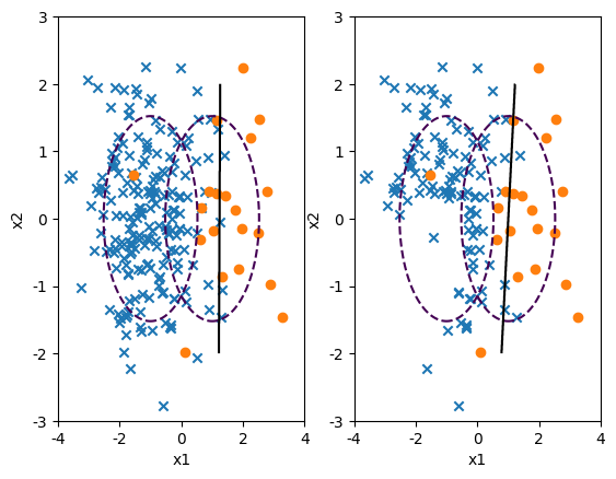
print(classification_report(y_imb, model_samp.predict(X_imb)))
#               precision    recall  f1-score   support
#
#          0.0       0.97      0.97      0.97       200
#          1.0       0.70      0.70      0.70        20
#
#     accuracy                           0.95       220
#    macro avg       0.83      0.83      0.83       220
# weighted avg 0.95 0.95 0.95 220- Neighbourhood Cleaning Rule
- CNN(Condensed Nearest Neighbour) 방법과 ENN(Edited Nearest Neighbours) 방법을 섞은 방법
- CNN: 1-nn 모형으로 분류되지 않는 데이터만 남기는 방법
- ENN: 다수 클래스 데이터 중 가장 가까운 k개의 데이터가 모두 또는 다수 클래스가 아니면 삭제하는 방법
- CNN(Condensed Nearest Neighbour) 방법과 ENN(Edited Nearest Neighbours) 방법을 섞은 방법
from imblearn.under_sampling import NeighbourhoodCleaningRule

X_samp, y_samp = NeighbourhoodCleaningRule(kind_sel="all", n_neighbors=5).fit_resample(X_imb, y_imb)

plt.subplot(121)
classification_result2(X_imb, y_imb)
plt.subplot(122)
model_samp = classification_result2(X_samp, y_samp)
print(classification_report(y_imb, model_samp.predict(X_imb)))
#               precision    recall  f1-score   support
#
#          0.0       0.99      0.93      0.96       200
#          1.0       0.56      0.95      0.70        20
#
#     accuracy                           0.93       220
#    macro avg       0.78      0.94      0.83       220
# weighted avg       0.96      0.93      0.94       220
Over-Sampling
- Random Over Sampler
- 소수 클래스의 데이터를 반복해서 넣는 방법
from imblearn.over_sampling import RandomOverSampler

X_samp, y_samp = RandomOverSampler(random_state=0).fit_resample(X_imb, y_imb)

plt.subplot(121)
classification_result2(X_imb, y_imb)
plt.subplot(122)
model_samp = classification_result2(X_samp, y_samp)
print(classification_report(y_imb, model_samp.predict(X_imb)))
#               precision    recall  f1-score   support
#
#          0.0       0.99      0.91      0.95       200
#          1.0       0.51      0.95      0.67        20
#
#     accuracy                           0.91       220
#    macro avg       0.75      0.93      0.81       220
# weighted avg 0.95 0.91 0.92 220- ADASYN(Adaptive Synthetic Sampling)
- 소수 클래스 데이터와 그 데이터에서 가장 가까운 k개의 소수 클래스 데이터 중 무작위로 선택된 데이터 사이의 직선상에 가상의 소수 클래스 데이터를 만드는 방법
from imblearn.over_sampling import ADASYN

X_samp, y_samp = ADASYN(random_state=0).fit_resample(X_imb, y_imb)

plt.subplot(121)
classification_result2(X_imb, y_imb)
plt.subplot(122)
model_samp = classification_result2(X_samp, y_samp)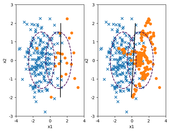
print(classification_report(y_imb, model_samp.predict(X_imb)))
#               precision    recall  f1-score   support
#
#          0.0       0.99      0.90      0.94       200
#          1.0       0.47      0.95      0.63        20
#
#     accuracy                           0.90       220
#    macro avg       0.73      0.92      0.79       220
# weighted avg 0.95 0.90 0.91 220- SMOTE(Synthetic Minority Over-Sampling Technique)
- ADASYN 방법처럼 데이터를 생성하지만, 생성된 데이터를 무조건 소수 클래스라고 하지 않고 분류 모형에 따라 분류한다.
from imblearn.over_sampling import SMOTE

X_samp, y_samp = SMOTE(random_state=4).fit_resample(X_imb, y_imb)

plt.subplot(121)
classification_result2(X_imb, y_imb)
plt.subplot(122)
model_samp = classification_result2(X_samp, y_samp)
print(classification_report(y_imb, model_samp.predict(X_imb)))
#               precision    recall  f1-score   support
#
#          0.0       0.99      0.91      0.95       200
#          1.0       0.50      0.90      0.64        20
#
#     accuracy                           0.91       220
#    macro avg       0.74      0.91      0.80       220
# weighted avg       0.94      0.91      0.92       220
2. Cross Validation
2-1. 교차 검증(Cross Validation)
train set으로 모델을 훈련하고 test set으로 모델을 검증하는 과정을 반복할 경우, 해당 test set에 overfitting하게 되기 때문에, 실제 데이터를 통해 예측을 수행하면 맞지 않는 경우가 발생한다. 이를 해결하기 위해 교차 검증을 수행한다.
2-2. 교차 검증 프로세스

2-3. 교차 검증 장단점
장점
- 모든 dataset을 훈련에 활용할 수 있다.
- 정확도를 향상시킬 수 있다.
- 데이터 부족으로 인한 underfitting을 방지할 수 있다.
- 모든 dataset을 평가에 활용할 수 있다.
- 평가에 사용되는 데이터 편중을 막을 수 있다.
- 평가 결과에 따라 좀 더 일반화된 모델을 만들 수 있다.
단점
- 반복 횟수가 많기 때문에 모델 훈련/평가 시간이 오래 걸린다.
2-4. 교차 검증 기법 종류
K-Fold
- 데이터를 k개의 데이터 폴드로 분할하고, 각 iteration마다 valid set을 다르게 할당하여 총 k개의 데이터 폴드 세트를 구성한다.
- 각 데이터 폴드 세트에 대해 나온 검증 결과들을 평균 내어 최종적인 검증 결과를 도출한다.
Stratified K-Fold
- 주로 classification 문제에서 사용하며, label의 분포가 각 클래스 별로 불균형을 이룰 때 사용한다.
- 각 valid set의 분포가 전체 데이터 세트가 가지고 있는 분포에 근사하게 된다.
2-5. 예제
데이터 로드
import numpy as np

from sklearn.model_selection import train_test_split
from sklearn import datasets

iris = datasets.load_iris()

X = iris.data
y = iris.target

X_train, X_test, y_train, y_test = train_test_split(X, y, test_size=0.4, random_state=0)
from sklearn import svm
clf = svm.SVC(kernel='linear', C=1)
clf.fit(X_train, y_train)
clf.score(X_test, y_test)
# 0.9666666666666667
교차 검증
- K-Fold
from sklearn.model_selection import KFold
from sklearn.metrics import accuracy_score

clf = svm.SVC(kernel='linear', C=1)

kf = KFold(n_splits=5, shuffle=True, random_state=0)

cv_test = kf.split(X_train)

n_iter = 0
accuracy_lst = []
for train_index, valid_index in cv_test:
    n_iter += 1

    train_x, valid_x = X_train[train_index], X_train[valid_index]
    train_y, valid_y = y_train[train_index], y_train[valid_index]

    clf.fit(train_x, train_y)

    pred = clf.predict(valid_x)

    accuracy = np.round(accuracy_score(valid_y, pred), 4)
    accuracy_lst.append(accuracy)

    print(f'{n_iter} 번째 K-fold 정확도: {accuracy}, 학습데이터 크기: {train_x.shape}, 검증데이터 크기: {valid_x.shape}')

print('-'*80)
print(f'교차 검증 정확도: {np.mean(accuracy_lst)} / 모델 평가: {clf.score(X_test, y_test)}')

# 1 번째 K-fold 정확도: 1.0, 학습데이터 크기: (72, 4), 검증데이터 크기: (18, 4)
# 2 번째 K-fold 정확도: 0.9444, 학습데이터 크기: (72, 4), 검증데이터 크기: (18, 4)
# 3 번째 K-fold 정확도: 0.9444, 학습데이터 크기: (72, 4), 검증데이터 크기: (18, 4)
# 4 번째 K-fold 정확도: 1.0, 학습데이터 크기: (72, 4), 검증데이터 크기: (18, 4)
# 5 번째 K-fold 정확도: 1.0, 학습데이터 크기: (72, 4), 검증데이터 크기: (18, 4)
# --------------------------------------------------------------------------------
# 교차 검증 정확도: 0.97776 / 모델 평가: 0.9666666666666667- Stratified K-Fold
from sklearn.model_selection import StratifiedKFold
import pandas as pd

df_train = pd.DataFrame(data=X_train, columns=iris.feature_names)
df_train['label'] = y_train

clf = svm.SVC(kernel='linear', C=1)

skf = StratifiedKFold(n_splits=5, shuffle=True, random_state=0)

n_iter = 0
accuracy_lst = []
for train_index, valid_index in skf.split(df_train, df_train['label']):
    n_iter += 1

    label_train = df_train['label'].iloc[train_index]
    label_valid = df_train['label'].iloc[valid_index]

    train_x, valid_x = X_train[train_index], X_train[valid_index]
    train_y, valid_y = y_train[train_index], y_train[valid_index]

    clf.fit(train_x, train_y)

    pred = clf.predict(valid_x)

    accuracy = np.round(accuracy_score(valid_y, pred), 4)
    accuracy_lst.append(accuracy)

    print(f'{n_iter} 번째 Stratified Stratified K-Fold 정확도: {accuracy}')

print('-'*60)
print(f'교차 검증 정확도: {np.mean(accuracy_lst)} / 모델 평가: {clf.score(X_test, y_test)}')

# 1 번째 Stratified Stratified K-Fold 정확도: 1.0
# 2 번째 Stratified Stratified K-Fold 정확도: 1.0
# 3 번째 Stratified Stratified K-Fold 정확도: 1.0
# 4 번째 Stratified Stratified K-Fold 정확도: 0.9444
# 5 번째 Stratified Stratified K-Fold 정확도: 1.0
# ------------------------------------------------------------
# 교차 검증 정확도: 0.98888 / 모델 평가: 0.8833333333333333
cross_val_predict()
- 모델을 통해 예측한 값들을 불러와 원하는 평가 계산 방법을 적용할 수 있도록 사용한다.
from sklearn.model_selection import cross_val_predict

clf = svm.SVC(kernel='linear', C=1)

predicts = cross_val_predict(clf, X_train, y_train, cv=5)

print(f'각 예측 결과: \n:{pd.Series(predicts)}')
# 각 예측 결과:
# :0     1
# 1     0
# 2     2
# 3     1
# 4     1
#      ..
# 85    0
# 86    2
# 87    1
# 88    2
# 89    0
# Length: 90, dtype: int64
cross_val_score()
- 평가 지표로 계산된 스코어에 대한 정보 확인
from sklearn.model_selection import cross_val_score

# K-Fold
clf = svm.SVC(kernel='linear', C=1)

scores = cross_val_score(clf, X_train, y_train, scoring='accuracy', cv=5)

print(f'각 검증 별 점수: \n{pd.Series(scores)}')
print(f'교차 검증 평균 점수: {np.mean(scores)}')
# 각 검증 별 점수:
# 0    1.000000
# 1    1.000000
# 2    1.000000
# 3    1.000000
# 4    0.944444
# dtype: float64
# 교차 검증 평균 점수: 0.9888888888888889

# Stratified K-Fold
skf = StratifiedKFold(n_splits=5, shuffle=True, random_state=0)

clf = svm.SVC(kernel='linear', C=1)

scores = cross_val_score(clf, X_train, y_train, scoring='accuracy', cv=skf)

print(f'각 검증 별 점수: \n{pd.Series(scores)}')
print(f'교차 검증 평균 점수: {np.mean(scores)}')
# 각 검증 별 점수:
# 0    1.000000
# 1    1.000000
# 2    1.000000
# 3    0.944444
# 4    1.000000
# dtype: float64
# 교차 검증 평균 점수: 0.9888888888888889
cross_validate()
- 여러 개의 평가지표를 사용하고 싶을 때 사용한다.
from sklearn.model_selection import cross_validate

clf = svm.SVC(kernel='linear', C=1)

result = cross_validate(clf, X_train, y_train, scoring='accuracy', cv=5, return_train_score=True)

print(f'각 검증 결과: \n: {pd.DataFrame(result)}')
# 각 검증 결과:
# :    fit_time  score_time  test_score  train_score
# 0  0.001987    0.001709    1.000000     0.986111
# 1  0.001429    0.000907    1.000000     1.000000
# 2  0.000993    0.000879    1.000000     0.986111
# 3  0.000971    0.000881    1.000000     0.986111
# 4  0.000959    0.000854    0.944444     1.000000
'SK네트웍스 Family AI캠프 10기 > Daily 회고' 카테고리의 다른 글
| 26일차. Deep Learning & PyTorch - Tensor (0) | 2025.02.17 |
|---|---|
| 25일차. AutoML & XAI & Pipeline (0) | 2025.02.14 |
| 23일차. Unsupervised Learning (0) | 2025.02.12 |
| 22일차. Supervised Learning - Classification & Ensemble & HPO (0) | 2025.02.11 |
| 21일차. Supervised Learning - Regression & Classification (0) | 2025.02.10 |


